dtreeviz : Decision Tree Visualization

Description

A python library for decision tree visualization and model interpretation. Currently supports scikit-learn, XGBoost, Spark MLlib, and LightGBM trees. With 1.3, we now provide one- and two-dimensional feature space illustrations for classifiers (any model that can answer predict_probab()); see below.

Authors:

Terence Parr, a professor in the University of San Francisco's data science program
Tudor Lapusan
Prince Grover

See How to visualize decision trees for deeper discussion of our decision tree visualization library and the visual design decisions we made.

Feedback

We welcome info from users on how they use dtreeviz, what features they'd like, etc... via email (to parrt) or via an issue.

Quick start

Jump right into the examples using this Colab notebook

Take a look in notebooks! Here we have a specific notebook for all supported ML libraries and more.

Discussion

Decision trees are the fundamental building block of gradient boosting machines and Random Forests(tm), probably the two most popular machine learning models for structured data. Visualizing decision trees is a tremendous aid when learning how these models work and when interpreting models. Unfortunately, current visualization packages are rudimentary and not immediately helpful to the novice. For example, we couldn't find a library that visualizes how decision nodes split up the feature space. It is also uncommon for libraries to support visualizing a specific feature vector as it weaves down through a tree's decision nodes; we could only find one image showing this.

So, we've created a general package for decision tree visualization and model interpretation, which we'll be using heavily in an upcoming machine learning book (written with Jeremy Howard).

The visualizations are inspired by an educational animation by R2D3; A visual introduction to machine learning. With dtreeviz, you can visualize how the feature space is split up at decision nodes, how the training samples get distributed in leaf nodes, how the tree makes predictions for a specific observation and more. These operations are critical to for understanding how classification or regression decision trees work. If you're not familiar with decision trees, check out fast.ai's Introduction to Machine Learning for Coders MOOC.

Install

Install anaconda3 on your system, if not already done.

You might verify that you do not have conda-installed graphviz-related packages installed because dtreeviz needs the pip versions; you can remove them from conda space by doing:

conda uninstall python-graphviz
conda uninstall graphviz

To install (Python >=3.6 only), do this (from Anaconda Prompt on Windows!):

pip install dtreeviz             # install dtreeviz for sklearn
pip install dtreeviz[xgboost]    # install XGBoost related dependency
pip install dtreeviz[pyspark]    # install pyspark related dependency
pip install dtreeviz[lightgbm]   # install LightGBM related dependency

This should also pull in the graphviz Python library (>=0.9), which we are using for platform specific stuff.

Limitations. Only svg files can be generated at this time, which reduces dependencies and dramatically simplifies install process.

Please email Terence with any helpful notes on making dtreeviz work (better) on other platforms. Thanks!

For your specific platform, please see the following subsections.

Mac

Make sure to have the latest XCode installed and command-line tools installed. You can run xcode-select --install from the command-line to install those if XCode is already installed. You also have to sign the XCode license agreement, which you can do with sudo xcodebuild -license from command-line. The brew install shown next needs to build graphviz, so you need XCode set up properly.

You need the graphviz binary for dot. Make sure you have latest version (verified on 10.13, 10.14):

brew reinstall graphviz

Just to be sure, remove dot from any anaconda installation, for example:

rm ~/anaconda3/bin/dot

From command line, this command

dot -Tsvg

should work, in the sense that it just stares at you without giving an error. You can hit control-C to escape back to the shell. Make sure that you are using the right dot as installed by brew:

$ which dot
/usr/local/bin/dot
$ ls -l $(which dot)
lrwxr-xr-x  1 parrt  wheel  33 May 26 11:04 /usr/local/bin/dot@ -> ../Cellar/graphviz/2.40.1/bin/dot
$

Limitations. Jupyter notebook has a bug where they do not show .svg files correctly, but Juypter Lab has no problem.

Linux (Ubuntu 18.04)

To get the dot binary do:

sudo apt install graphviz

Limitations. The view() method works to pop up a new window and images appear inline for jupyter notebook but not jupyter lab (It gets an error parsing the SVG XML.) The notebook images also have a font substitution from the Arial we use and so some text overlaps. Only .svg files can be generated on this platform.

Windows 10

(Make sure to pip install graphviz, which is common to all platforms, and make sure to do this from Anaconda Prompt on Windows!)

Download graphviz-2.38.msi and update your Path environment variable. Add C:\Program Files (x86)\Graphviz2.38\bin to User path and C:\Program Files (x86)\Graphviz2.38\bin\dot.exe to System Path. It's windows so you might need a reboot after updating that environment variable. You should see this from the Anaconda Prompt:

(base) C:\Users\Terence Parr>where dot
C:\Program Files (x86)\Graphviz2.38\bin\dot.exe

(Do not use conda install -c conda-forge python-graphviz as you get an old version of graphviz python library.)

Verify from the Anaconda Prompt that this works (capital -V not lowercase -v):

dot -V

If it doesn't work, you have a Path problem. I found the following test programs useful. The first one sees if Python can find dot:

import os
import subprocess
proc = subprocess.Popen(['dot','-V'])
print( os.getenv('Path') )

The following version does the same thing except uses graphviz Python libraries backend support utilities, which is what we use in dtreeviz:

import graphviz.backend as be
cmd = ["dot", "-V"]
stdout, stderr = be.run(cmd, capture_output=True, check=True, quiet=False)
print( stderr )

If you are having issues with run command you can try copying the following files from: https://github.com/xflr6/graphviz/tree/master/graphviz.

Place them in the AppData\Local\Continuum\anaconda3\Lib\site-packages\graphviz folder.

Clean out the pycache directory too.

Jupyter Lab and Jupyter notebook both show the inline .svg images well.

Verify graphviz installation

Try making text file t.dot with content digraph T { A -> B } (paste that into a text editor, for example) and then running this from the command line:

dot -Tsvg -o t.svg t.dot

That should give a simple t.svg file that opens properly. If you get errors from dot, it will not work from the dtreeviz python code. If it can't find dot then you didn't update your PATH environment variable or there is some other install issue with graphviz.

Limitations

Finally, don't use IE to view .svg files. Use Edge as they look much better. I suspect that IE is displaying them as a rasterized not vector images. Only .svg files can be generated on this platform.

Usage

dtree: Main function to create decision tree visualization. Given a decision tree regressor or classifier, creates and returns a tree visualization using the graphviz (DOT) language.

Required libraries

Basic libraries and imports that will (might) be needed to generate the sample visualizations shown in examples below.

from sklearn.datasets import *
from sklearn import tree
from dtreeviz.trees import *

Regression decision tree

The default orientation of tree is top down but you can change it to left to right using orientation="LR". view() gives a pop up window with rendered graphviz object.

regr = tree.DecisionTreeRegressor(max_depth=2)
boston = load_boston()
regr.fit(boston.data, boston.target)

viz = dtreeviz(regr,
               boston.data,
               boston.target,
               target_name='price',
               feature_names=boston.feature_names)
              
viz.view()

Classification decision tree

An additional argument of class_names giving a mapping of class value with class name is required for classification trees.

classifier = tree.DecisionTreeClassifier(max_depth=2)  # limit depth of tree
iris = load_iris()
classifier.fit(iris.data, iris.target)

viz = dtreeviz(classifier, 
               iris.data, 
               iris.target,
               target_name='variety',
               feature_names=iris.feature_names, 
               class_names=["setosa", "versicolor", "virginica"]  # need class_names for classifier
              )  
              
viz.view()

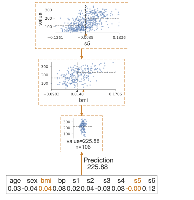
Prediction path

Highlights the decision nodes in which the feature value of single observation passed in argument X falls. Gives feature values of the observation and highlights features which are used by tree to traverse path.

regr = tree.DecisionTreeRegressor(max_depth=2)  # limit depth of tree
diabetes = load_diabetes()
regr.fit(diabetes.data, diabetes.target)
X = diabetes.data[np.random.randint(0, len(diabetes.data)),:]  # random sample from training

viz = dtreeviz(regr,
               diabetes.data, 
               diabetes.target, 
               target_name='value', 
               orientation ='LR',  # left-right orientation
               feature_names=diabetes.feature_names,
               X=X)  # need to give single observation for prediction
              
viz.view()

If you want to visualize just the prediction path, you need to set parameter show_just_path=True

dtreeviz(regr,
        diabetes.data, 
        diabetes.target, 
        target_name='value', 
        orientation ='TD',  # top-down orientation
        feature_names=diabetes.feature_names,
        X=X, # need to give single observation for prediction
        show_just_path=True     
        )

Explain prediction path

These visualizations are useful to explain to somebody, without machine learning skills, why your model made that specific prediction.
In case of explanation_type=plain_english, it searches in prediction path and find feature value ranges.

X = dataset[features].iloc[10]
print(X)
Pclass              3.0
Age                 4.0
Fare               16.7
Sex_label           0.0
Cabin_label       145.0
Embarked_label      2.0

print(explain_prediction_path(tree_classifier, X, feature_names=features, explanation_type="plain_english"))
2.5 <= Pclass 
Age < 36.5
Fare < 23.35
Sex_label < 0.5

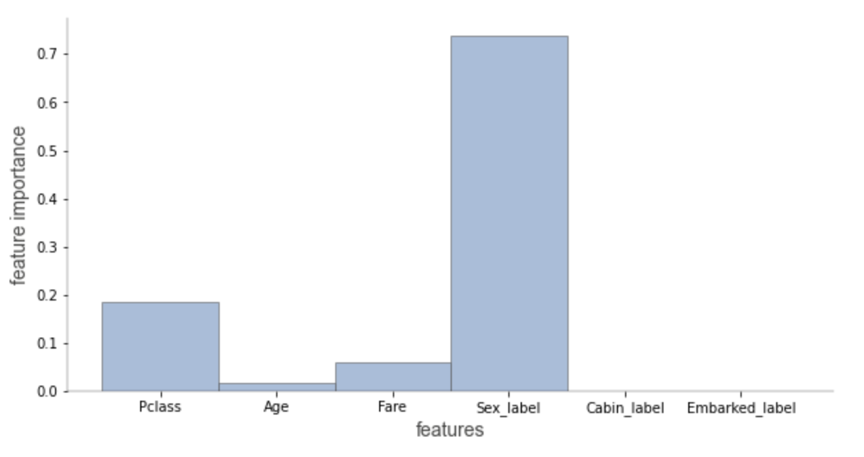
In case of explanation_type=sklearn_default (available only for scikit-learn), we can visualize the features' importance involved in prediction path only. Features' importance is calculated based on mean decrease in impurity.
Check Beware Default Random Forest Importances article for a comparison between features' importance based on mean decrease in impurity vs permutation importance.

explain_prediction_path(tree_classifier, X, feature_names=features, explanation_type="sklearn_default")

Decision tree without scatterplot or histograms for decision nodes

Simple tree without histograms or scatterplots for decision nodes. Use argument fancy=False

classifier = tree.DecisionTreeClassifier(max_depth=4)  # limit depth of tree
cancer = load_breast_cancer()
classifier.fit(cancer.data, cancer.target)

viz = dtreeviz(classifier,
              cancer.data,
              cancer.target,
              target_name='cancer',
              feature_names=cancer.feature_names, 
              class_names=["malignant", "benign"],
              fancy=False )  # fance=False to remove histograms/scatterplots from decision nodes
              
viz.view()

For more examples and different implementations, please see the jupyter notebook full of examples.

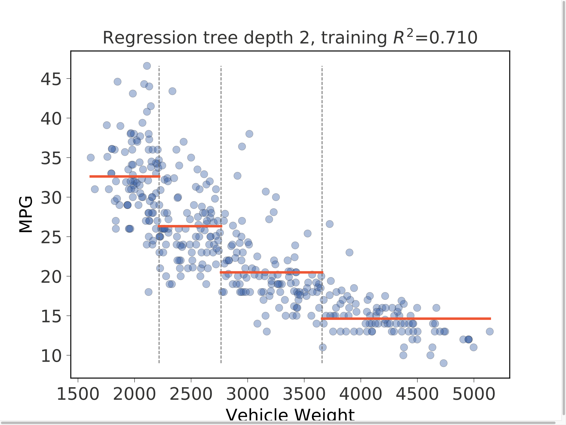
Regression univariate feature-target space

import pandas as pd
import matplotlib.pyplot as plt
from sklearn.tree import DecisionTreeRegressor
from dtreeviz.trees import *

df_cars = pd.read_csv("cars.csv")
X, y = df_cars[['WGT']], df_cars['MPG']

dt = DecisionTreeRegressor(max_depth=3, criterion="mae")
dt.fit(X, y)

fig = plt.figure()
ax = fig.gca()
rtreeviz_univar(dt, X, y, 'WGT', 'MPG', ax=ax)
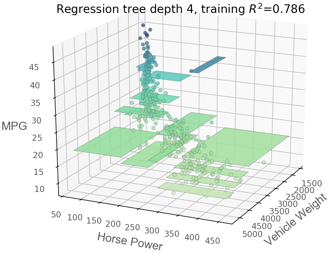
plt.show()

Regression bivariate feature-target space

from mpl_toolkits.mplot3d import Axes3D
from sklearn.tree import DecisionTreeRegressor
from dtreeviz.trees import *

df_cars = pd.read_csv("cars.csv")
X = df_cars[['WGT','ENG']]
y = df_cars['MPG']

dt = DecisionTreeRegressor(max_depth=3, criterion="mae")
dt.fit(X, y)

figsize = (6,5)
fig = plt.figure(figsize=figsize)
ax = fig.add_subplot(111, projection='3d')

t = rtreeviz_bivar_3D(dt,
                      X, y,
                      feature_names=['Vehicle Weight', 'Horse Power'],
                      target_name='MPG',
                      fontsize=14,
                      elev=20,
                      azim=25,
                      dist=8.2,
                      show={'splits','title'},
                      ax=ax)
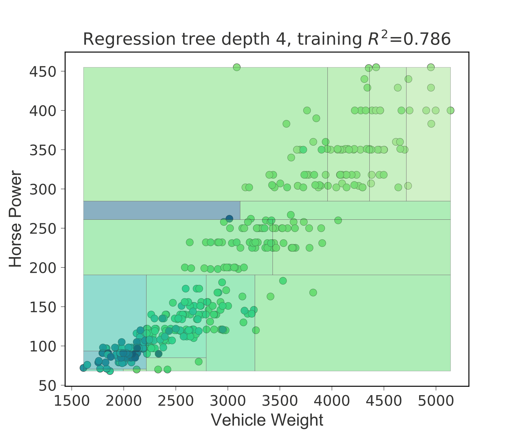
plt.show()

Regression bivariate feature-target space heatmap

from sklearn.tree import DecisionTreeRegressor
from dtreeviz.trees import *

df_cars = pd.read_csv("cars.csv")
X = df_cars[['WGT','ENG']]
y = df_cars['MPG']

dt = DecisionTreeRegressor(max_depth=3, criterion="mae")
dt.fit(X, y)

t = rtreeviz_bivar_heatmap(dt,
                           X, y,
                           feature_names=['Vehicle Weight', 'Horse Power'],
                           fontsize=14)

plt.show()

Classification univariate feature-target space

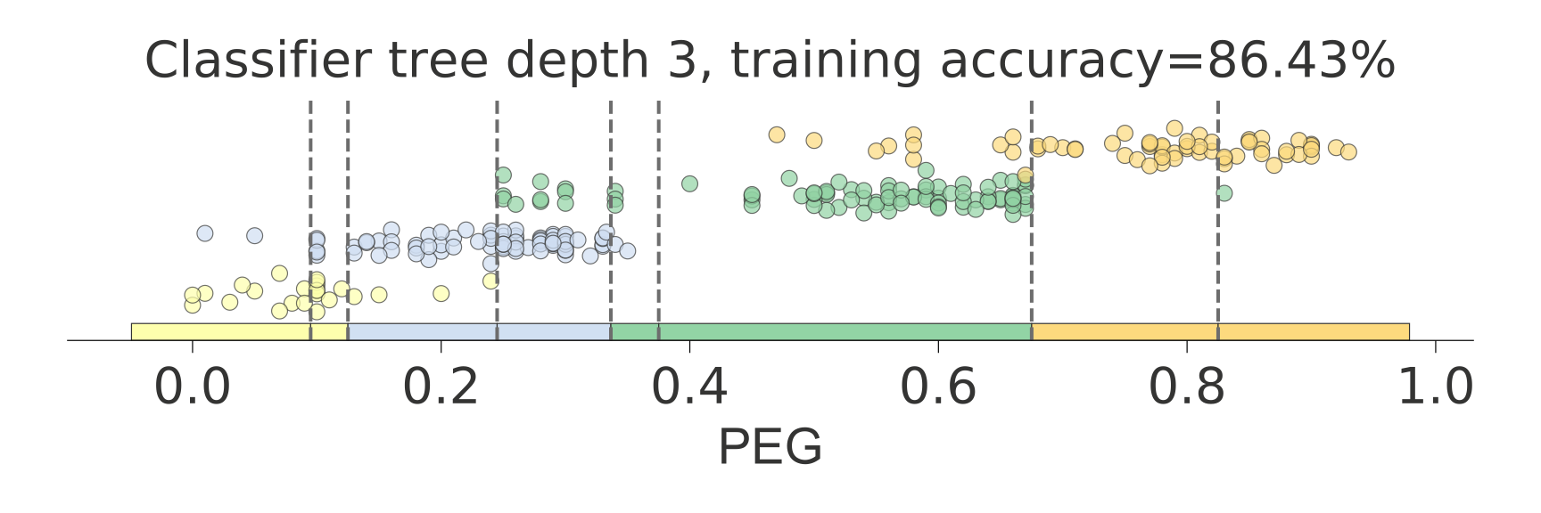
from sklearn.tree import DecisionTreeClassifier
from dtreeviz.trees import *

know = pd.read_csv("knowledge.csv")
class_names = ['very_low', 'Low', 'Middle', 'High']
know['UNS'] = know['UNS'].map({n: i for i, n in enumerate(class_names)})

X = know[['PEG']]
y = know['UNS']

dt = DecisionTreeClassifier(max_depth=3)
dt.fit(X, y)

ct = ctreeviz_univar(dt, X, y,
                     feature_names = ['PEG'],
                     class_names=class_names,
                     target_name='Knowledge',
                     nbins=40, gtype='strip',
                     show={'splits','title'})
plt.tight_layout()
plt.show()

Classification bivariate feature-target space

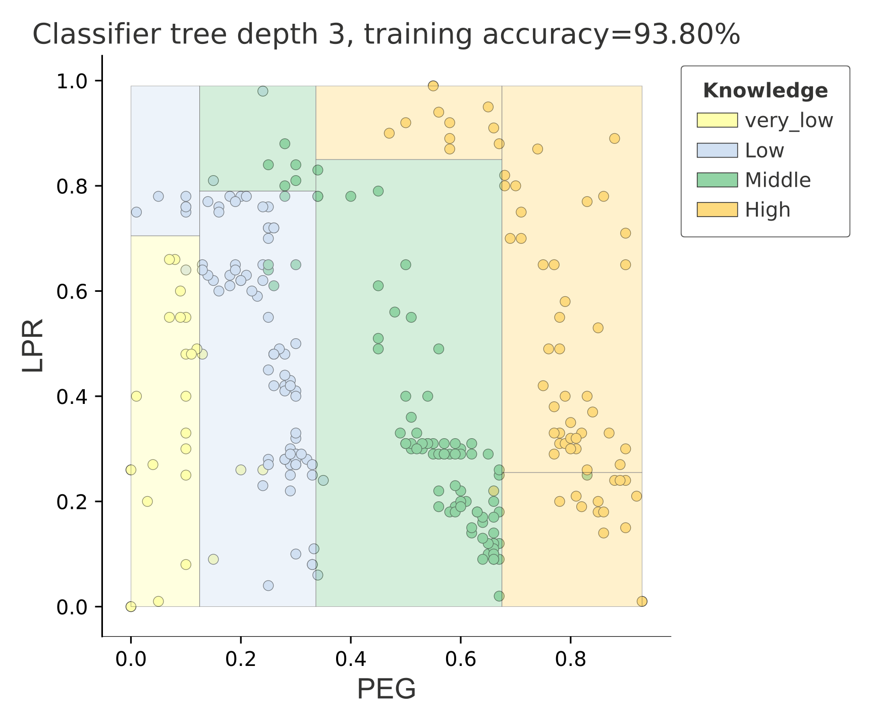
from sklearn.tree import DecisionTreeClassifier
from dtreeviz.trees import *

know = pd.read_csv("knowledge.csv")
print(know)
class_names = ['very_low', 'Low', 'Middle', 'High']
know['UNS'] = know['UNS'].map({n: i for i, n in enumerate(class_names)})

X = know[['PEG','LPR']]
y = know['UNS']

dt = DecisionTreeClassifier(max_depth=3)
dt.fit(X, y)

ct = ctreeviz_bivar(dt, X, y,
                    feature_names = ['PEG','LPR'],
                    class_names=class_names,
                    target_name='Knowledge')
plt.tight_layout()
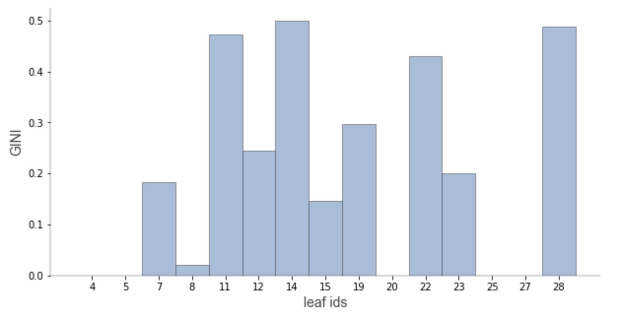
plt.show()

Leaf node purity

Leaf purity affects prediction confidence.
For classification leaf purity is calculated based on majority target class (gini, entropy) and for regression is calculated based on target variance values.
Leaves with low variance among the target values (regression) or an overwhelming majority target class (classification) are much more reliable predictors. When we have a decision tree with a high depth, it can be difficult to get an overview about all leaves purities. That's why we created a specialized visualization only for leaves purities.

display_type can take values 'plot' (default), 'hist' or 'text'

viz_leaf_criterion(tree_classifier, display_type = "plot")

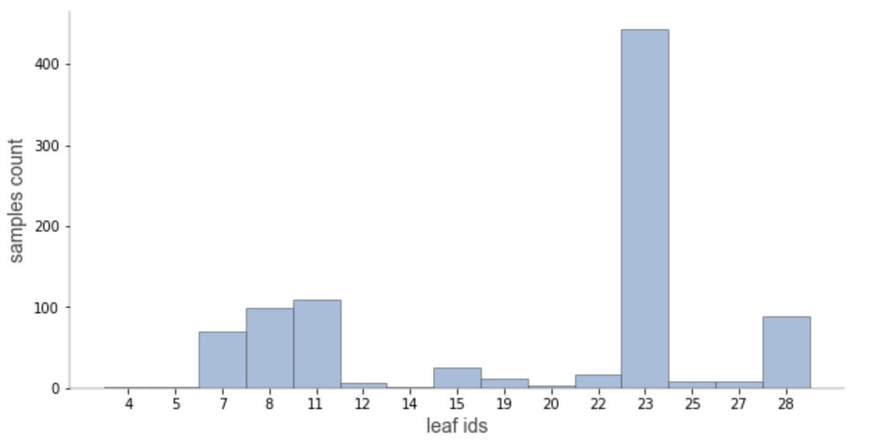
Leaf node samples

It's also important to take a look at the number of samples from leaves. For example, we can have a leaf with a good purity but very few samples, which is a sign of overfitting. The ideal scenario would be to have a leaf with good purity which is based on a significant number of samples.

display_type can take values 'plot' (default), 'hist' or 'text'

viz_leaf_samples(tree_classifier, dataset[features], display_type='plot')

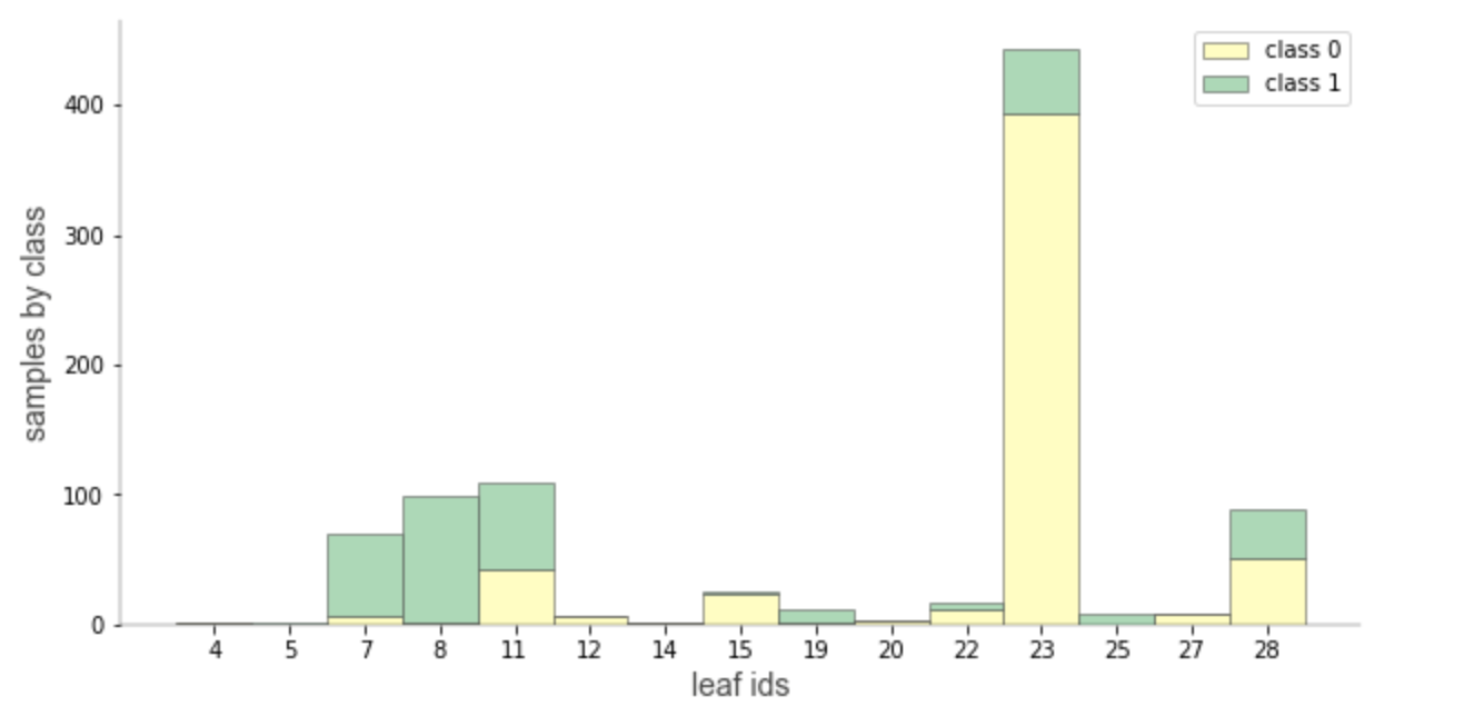
Leaf node samples for classification

This is a specialized visualization for classification. It helps also to see the distribution of target class values from leaf samples.

ctreeviz_leaf_samples(tree_classifier, dataset[features], dataset[target])

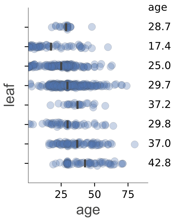
Leaf plots

Visualize leaf target distribution for regression decision trees.

viz_leaf_target(tree_regressor, dataset[features_reg], dataset[target_reg], features_reg, target_reg)

Classification boundaries in feature space

With 1.3, we have introduced method clfviz() that illustrates one and two-dimensional feature space for classifiers, including colors the represent probabilities, decision boundaries, and misclassified entities. This method works with any model that answers method predict_proba() (and we also support Keras), so any model from scikit-learn should work. If you let us know about incompatibilities, we can support more models. There are lots of options would you can check out in the api documentation. See classifier-decision-boundaries.ipynb and classifier-boundary-animations.ipynb.

clfviz(rf, X, y, feature_names=['x1', 'x2'], markers=['o','X','s','D'], target_name='smiley')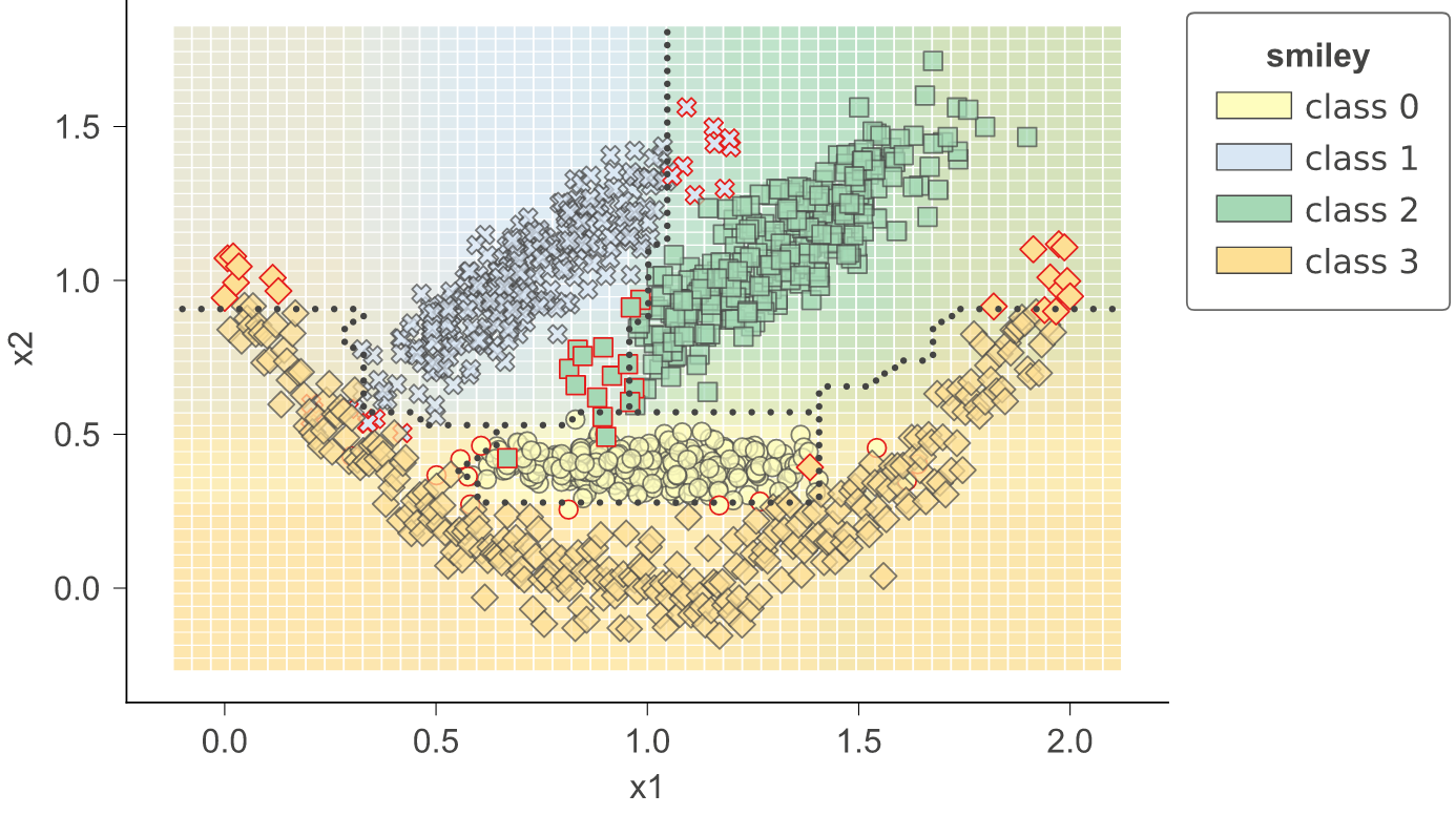

clfviz(rf,x,y,feature_names=['f27'],target_name='cancer')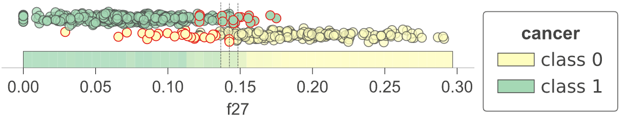

clfviz(rf,x,y,
       feature_names=['x2'],
       target_name = 'smiley',
       colors={'scatter_marker_alpha':.2})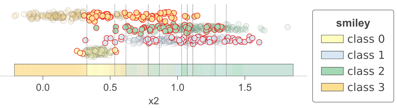

Sometimes it's helpful to see animations that change some of the hyper parameters. If you look in notebook classifier-boundary-animations.ipynb, you will see code that generates animations such as the following (animated png files):

Visualization methods setup

Starting with dtreeviz 1.0 version, we refactored the concept of ShadowDecTree. If we want to add a new ML library in dtreeviz, we just need to add a new implementation of ShadowDecTree API, like ShadowSKDTree, ShadowXGBDTree or ShadowSparkTree.

Initializing a ShadowSKDTree object:

sk_dtree = ShadowSKDTree(tree_classifier, dataset[features], dataset[target], features, target, [0, 1])

Once we have the object initialized, we can used it to create all the visualizations, like :

dtreeviz(sk_dtree)

viz_leaf_samples(sk_dtree)

viz_leaf_criterion(sk_dtree)

In this way, we reduced substantially the list of parameters required for each visualization and it's also more efficient in terms of computing power.

You can check the notebooks section for more examples of using ShadowSKDTree, ShadowXGBDTree or ShadowSparkTree.

Install dtreeviz locally

Make sure to follow the install guidelines above.

To push the dtreeviz library to your local egg cache (force updates) during development, do this (from anaconda prompt on Windows):

python setup.py install -f

E.g., on Terence's box, it add /Users/parrt/anaconda3/lib/python3.6/site-packages/dtreeviz-0.3-py3.6.egg.

Customize colors

Each function has an optional parameter colors which allows passing a dictionary of colors which is used in the plot. For an example of each parameter have a look at this notebook.

Example

dtreeviz.trees.dtreeviz(regr,
                        boston.data,
                        boston.target,
                        target_name='price',
                        feature_names=boston.feature_names,
                        colors={'scatter_marker': '#00ff00'})

would paint the scatter (dots) in red.

Parameters

The colors are defined in colors.py, all options and default parameters are shown below.

    COLORS = {'scatter_edge': GREY,         
              'scatter_marker': BLUE,
              'split_line': GREY,
              'mean_line': '#f46d43',
              'axis_label': GREY,
              'title': GREY,
              'legend_title': GREY,
              'legend_edge': GREY,
              'edge': GREY,
              'color_map_min': '#c7e9b4',
              'color_map_max': '#081d58',
              'classes': color_blind_friendly_colors,
              'rect_edge': GREY,
              'text': GREY,
              'highlight': HIGHLIGHT_COLOR,
              'wedge': WEDGE_COLOR,
              'text_wedge': WEDGE_COLOR,
              'arrow': GREY,
              'node_label': GREY,
              'tick_label': GREY,
              'leaf_label': GREY,
              'pie': GREY,
              }

The color needs be in a format matplotlib can interpret, e.g. a html hex like '#eeefff' .

classes needs to be a list of lists of colors with a minimum length of your number of colors. The index is the number of classes and the list with this index needs to have the same amount of colors.

Useful Resources

How to visualize decision trees
How to explain gradient boosting
The Mechanics of Machine Learning
Animation by R2D3
A visual introductionn to machine learning
fast.ai's Introduction to Machine Learning for Coders MOOC
Stef van den Elzen's Interactive Construction, Analysis and Visualization of Decision Trees
Some similar feature-space visualizations in Towards an effective cooperation of the user and the computer for classification, SIGKDD 2000
Beautiful Decisions: Inside BigML’s Decision Trees
"SunBurst" approach to tree visualization: An evaluation of space-filling information visualizations for depicting hierarchical structures

Authors

See also the list of contributors who participated in this project.

License

This project is licensed under the terms of the MIT license, see LICENSE.

Deploy

$ python setup.py sdist upload

Cheap and reliable Node.js hosting starts at $3/month, and $1/month static HTML hosting

parrt / Dtreeviz

Programming Languages

Labels

Projects that are alternatives of or similar to Dtreeviz