ropensci / Osmplotr

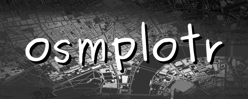
R package to produce visually impressive customisable images of OpenStreetMap (OSM) data downloaded internally from the overpass api. The above map was produced directly from osmplotr with no further modification. This README briefly demonstrates the following functionality:

1. Quick Introduction

2. Installation

3. A Simple Map

4. Highlighting Selected Areas

5. Highlighting Clusters

6. Highlighting Areas Bounded by Named Highways

7. Data Surfaces

8. Gallery

1. Quick Introduction

But first the easy steps to map making:

1. Specify the bounding box for the desired region

   bbox <- get_bbox (c(-0.15, 51.5, -0.10, 51.52))
   

2. Download the desired data—in this case, all building perimeters.

   dat_B <- extract_osm_objects (key = 'building', bbox = bbox)
   

3. Initiate an osm_basemap with desired background (bg) colour

   map <- osm_basemap (bbox = bbox, bg = 'gray20')
   

4. Overlay objects on plot in the desired colour.

   map <- add_osm_objects (map, dat_B, col = 'gray40')
   

5. Print the map to graphics device of choice

   print_osm_map (map)
   

2. Installation

First install the package

install.packages ('osmplotr')

or the development version

devtools::install_github ('ropensci/osmplotr')

And then load it in the usual way

library (osmplotr)

3. A Simple Map

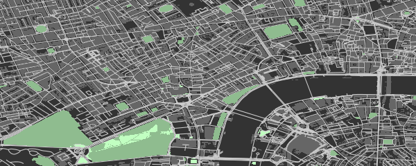
Simple maps can be made by overlaying different kinds of OSM data in different colours:

dat_H <- extract_osm_objects (key = 'highway', bbox = bbox)
dat_P <- extract_osm_objects (key = 'park', bbox = bbox)
dat_G <- extract_osm_objects (key = 'landuse', value = 'grass', bbox = bbox)

map <- osm_basemap (bbox = bbox, bg = 'gray20')
map <- add_osm_objects (map, dat_B, col = 'gray40')
map <- add_osm_objects (map, dat_H, col = 'gray80')
map <- add_osm_objects (map, dat_P, col = 'darkseagreen')
map <- add_osm_objects (map, dat_G, col = 'darkseagreen1')
print_osm_map (map)

4. Highlighting Selected Areas

osmplotr is primarily intended as a data visualisation tool, particularly through enabling selected regions to be highlighted. Regions can be defined according to simple point boundaries:

pts <- sp::SpatialPoints (cbind (c (-0.115, -0.13, -0.13, -0.115),
                             c (51.505, 51.505, 51.515, 51.515)))

OSM objects within the defined regions can then be highlighted with different colour schemes. cols defines colours for each group (with only one here), while bg defines the colour of the remaining, background area.

map <- osm_basemap (bbox = bbox, bg = 'gray20')
map <- add_osm_groups (map, dat_B, groups = pts, cols = 'orange', bg = 'gray40')
map <- add_osm_objects (map, london$dat_P, col = 'darkseagreen1')
map <- add_osm_groups (map, london$dat_P, groups = pts, cols = 'darkseagreen1',
                   bg = 'darkseagreen', boundary = 0)
print_osm_map (map)

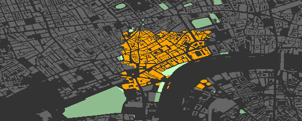
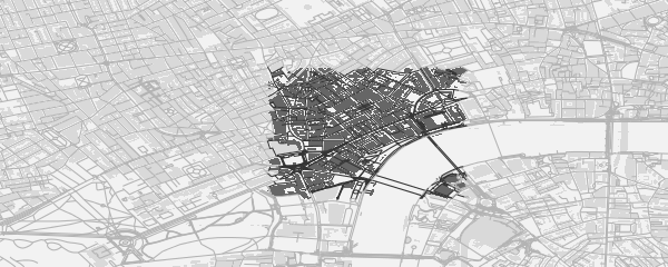
Note the border = 0 argument on the last call divides the park polygons precisely along the border. The same map highlighted in dark-on-light:

map <- osm_basemap (bbox = bbox, bg = 'gray95')
map <- add_osm_groups (map, dat_B, groups = pts, cols = 'gray40', bg = 'gray85')
map <- add_osm_groups (map, dat_H, groups = pts, cols = 'gray20', bg = 'gray70')
print_osm_map (map)

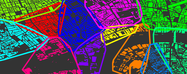
5. Highlighting Clusters

add_osm_groups also enables plotting an entire region as a group of spatially distinct clusters of defined colours. Groups can be defined by simple spatial points denoting their centres:

set.seed (2)
ngroups <- 12
x <- bbox [1, 1] + runif (ngroups) * diff (bbox [1, ])
y <- bbox [2, 1] + runif (ngroups) * diff (bbox [2, ])
groups <- cbind (x, y)
groups <- apply (groups, 1, function (i)
              sp::SpatialPoints (matrix (i, nrow = 1, ncol = 2)))

Calling add_osm_groups with no bg argument forces all points lying outside those defined groups to be allocated to the nearest groups, and thus produces an inclusive grouping extending across an entire region.

map <- osm_basemap (bbox = bbox, bg = 'gray20')
map <- add_osm_groups (map, dat_B, groups = groups,
                       cols = rainbow (length (groups)), border_width = 2)
print_osm_map (map)

6. Highlighting Areas Bounded by Named Highways

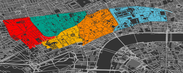
An alternative way of defining highlighted groups is by naming the highways encircling desired regions.

# These highways extend beyond the previous, smaller bbox
bbox_big <- get_bbox (c(-0.15, 51.5, -0.10, 51.52))
highways <- c ('Davies.St', 'Berkeley.Sq', 'Berkeley.St', 'Piccadilly',
               'Regent.St', 'Oxford.St')
highways1 <- connect_highways (highways = highways, bbox = bbox_big)
highways <- c ('Regent.St', 'Oxford.St', 'Shaftesbury')
highways2 <- connect_highways (highways = highways, bbox = bbox_big)
highways <- c ('Piccadilly', 'Shaftesbury.Ave', 'Charing.Cross.R',
               'Saint.Martin', 'Trafalgar.Sq', 'Cockspur.St',
               'Pall.Mall', 'St.James')
highways3 <- connect_highways (highways = highways, bbox = bbox_big)
highways <- c ('Charing.Cross', 'Duncannon.St', 'Strand', 'Aldwych',
               'Kingsway', 'High.Holborn', 'Shaftesbury.Ave')
highways4 <- connect_highways (highways = highways, bbox = bbox_big)
highways <- c ('Kingsway', 'Holborn', 'Farringdon.St', 'Strand',
               'Fleet.St', 'Aldwych')
highways5 <- connect_highways (highways = highways, bbox = bbox_big)
groups <- list (highways1, highways2, highways3, highways4, highways5)

And then passing these lists of groups returned by connect_highways to add_osm_groups, this time with some Wes Anderson flair.

map <- osm_basemap (bbox = bbox, bg = 'gray20')
library (wesanderson)
cols <- wes_palette ('Darjeeling', 5)
map <- add_osm_groups (map, dat_B, groups = groups, boundary = 1,
                       cols = cols, bg = 'gray40', colmat = FALSE)
map <- add_osm_groups (map, dat_H, groups = groups, boundary = 0,
                       cols = cols, bg = 'gray70', colmat = FALSE)
print_osm_map (map)

7. Data Surfaces

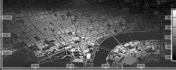
Finally, osmplotr contains a function add_osm_surface that spatially interpolates a given set of spatial data points and colours OSM objects according to a specified colour gradient. This is illustrated here with the volcano data projected onto the bbox.

x <- seq (bbox [1, 1], bbox [1, 2], length.out = dim (volcano)[1])
y <- seq (bbox [2, 1], bbox [2, 2], length.out = dim (volcano)[2])
xy <- cbind (rep (x, dim (volcano) [2]), rep (y, each = dim (volcano) [1]))
z <- as.numeric (volcano)
dat <- data.frame (x = xy [, 1], y = xy [, 2], z = z)

map <- osm_basemap (bbox = bbox, bg = 'gray20')
cols <- gray (0:50 / 50)
map <- add_osm_surface (map, dat_B, dat = dat, cols = cols)
# Darken cols by ~20%
map <- add_osm_surface (map, dat_H, dat = dat,
                        cols = adjust_colours (cols, -0.2))
map <- add_colourbar (map, cols = cols, zlims = range (volcano))
map <- add_axes (map)
print_osm_map (map)

8. Gallery

Got a nice osmplotr map? Please contribute in one of the following ways:

1. Fork repo, add link to README.md/.Rmd, and send pull request; or

2. Open issue with details; or

3. Send email to address in DESCRIPTION.

See package vignettes (basic maps and data maps) for a lot more detail and further capabilities of osmplotr. Please note that this project is released with a Contributor Code of Conduct. By participating in this project you agree to abide by its terms.