Vehicle Detection and Tracking

Introduction

Here we are going to use some hallmark techniques of classical computer vision (i.e. no deep learning) to see how far we can get in detecting and tracking vehicles. These are

• a Histogram of Oriented Gradients (HOG) feature extraction on a labeled training set of images and train a Linear SVM classifier.
• a color transform and binned color features, as well as histograms of color, to combine the HOG feature vector with other classical computer vision approaches
• a sliding-window technique to search for cars with the trained SVM
• creating a heatmap of recurring detections in subsequent framens of a video stream to reject outliers and follow detected vehicles.
• finally we will compare our results to those of a YOLOv2, a blazingly fast neural network for object detection

This pipeline is then used to draw bounding boxes around the cars in the video.

Getting Started

• Clone the project and create directories vehicles and non-vehicles.
• Download images from the links given below and put them into subfolders below vehicles and non-vehicles.
• exploration.ipynb splits the data into training, validation and test set and saves them in a pickle file.
• HOG_Classify.ipynb trains an SVM to detect cars and non-cars. All classifier data is saved in a pickle file.
• search_classify.ipynb implements a sliding window search for cars, including false positive filtering and applies the classifier to a video What follows describes the pipeline above in more detail.

Please see the rubric points

Data Exploration

Labeled images were taken from the GTI vehicle image database GTI, the KITTI vision benchmark suite, and examples extracted from the project video itself. All images are 64x64 pixels. A third data set released by Udacity was not used here. In total there are 8792 images of vehicles and 9666 images of non vehicles. Thus the data is slightly unbalanced with about 10% more non vehicle images than vehicle images. Images of the GTI data set are taken from video sequences which needed to be addressed in the separation into training and test set. 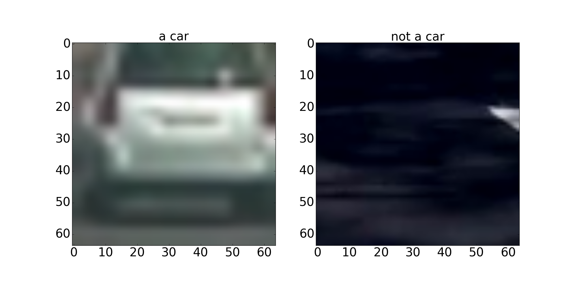Shown below is an example of each class (vehicle, non-vehicle) of the data set. The data set is explored in the notebook exploration.ipynb

Histogram of Oriented Gradients (HOG)

Extraction of HOG, color and spatial features

Due to the temporal correlation in the video sequences, the training set was divided as follows: the first 70% of any folder containing images was assigned to be the training set, the next 20% the validation set and the last 10% the test set. In the process of generating HOG features all training, validation and test images were normalized together and subsequently split again into training, test and validation set. Each set was shuffled individually. The code for this step is contained in the first six cells of the IPython notebook HOG_Classify.ipynb. I explored different color spaces and different skimage.hog() parameters (orientations, pixels_per_cell, and cells_per_block).
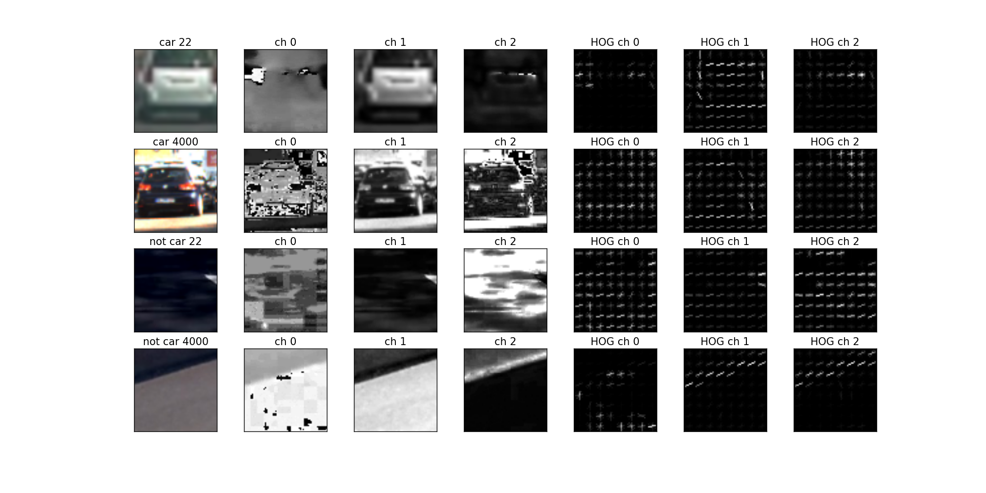
I selected a few images from each of the two classes and displayed them to see what the skimage.hog() output looks like. Here is an example using the HLS color space and HOG parameters of orient=9, pixels_per_cell=(16, 16) and cells_per_block=(2, 2):

Choice of parameters and channels for HOG

I experimented with a number of different combinations of color spaces and HOG parameters and trained a linear SVM using different combinations of HOG features extracted from the color channels. For HLS color space the L-channel appears to be most important, followed by the S channel. I discarded RGB color space, for its undesirable properties under changing light conditions. YUV and YCrCb also provided good results, but proved to be unstable when all channels were used. There was relatively little variation in the final accuracy when running the SVM with some of the individual channels of HSV,HLS and LUV. I finally settled with HLS space and a low value of pixels_per_cell=(8,8). Using larger values of than orient=9 did not have a striking effect and only increased the feature vector. Similarly, using values larger than cells_per_block=(2,2) did not improve results, which is why these values were chosen.

Training a linear SVM on the final choice of features

I trained a linear SVM using all channels of images converted to HLS space. I included spatial features color features as well as all three HLS channels, because using less than all three channels reduced the accuracy considerably. The final feature vector has a length of 6156 elements, most of which are HOG features. For color binning patches of spatial_size=(16,16) were generated and color histograms were implemented using hist_bins=32 used. After training on the training set this resulted in a validation and test accuracy of 98%. The average time for a prediction (average over a hundred predictions) turned out to be about 3.3ms on an i7 processor, thus allowing a theoretical bandwidth of 300Hz. A realtime application would therfore only feasible if several parts of the image are examined in parallel in a similar time. The sliding window search described below is an embarrassingly parallel task and corresponding speedups can be expected, but implementing it is beyond the scope of this project. Using just the L channel reduced the feature vector to about a third, while test and validation accuracy dropped to about 94.5% each. Unfortunately, the average time for a prediction remained about the same as before. The classifier used was LinearSVC taken from the scikit-learn package. Despite the high accuracy there is a systematic error as can be seen from investigating the false positive detections. The false positives include frequently occuring features, such as side rails, line line markers etc. Shown below are some examples that illustrate this problem.

Sliding Window Search

Implementation of the sliding window search

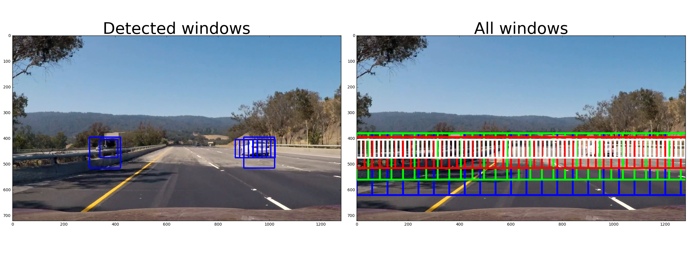
In the file search_classify.ibynb I segmented the image into 4 partially overlapping zones with different sliding window sizes to account for different distances. The window sizes are 240,180,120 and 70 pixels for each zone. Within each zone adjacent windows have an ovelap of 75%, as illustrated below. The search over all zones is implemented in the search_all_scales(image) function. Using even slightly less than 75% overlap resulted in an unacceptably large number of false negatives.

Search examples

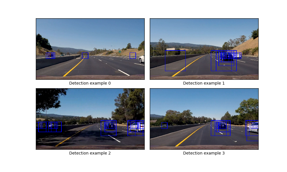
The final classifier uses four scales and HOG features from all 3 channels of images in HLS space. The feature vector contains also spatially binned color and histograms of color features False positives occured more frequently for pixels_per_cell=8 compared to pixels_per_cell=16, but nevertheless produced better results when applied to the video. The false positives were filtered out by using a heatmap approach as described below. Here are some typical examples of detections

False positives occur on the side of the road, but also simple lane lines get detected as cars from time to time. Cars driving in the opposite direction also get detected in so far as a significant portion is visible.

Video Implementation

Applying the developed pipeline to a video is the logical next step. An example of applying the pipeline to a video can be found here

False positive filtering by a heatmap

In the file search_classify.ipynb the class BoundingBoxes implements a FIFO queue that stores the bounding boxes of the last n frames. For every frame the (possbly empty) list of detected bounding boxes gets added to the beginning of the queue, while the oldest list of bounding boxes falls out. This queue is then used in the processing of the video and always contains the bounding boxes of the last n=20 frames. On these a threshold of 20 was applied, which suppresses also false positives from detected lane lines. 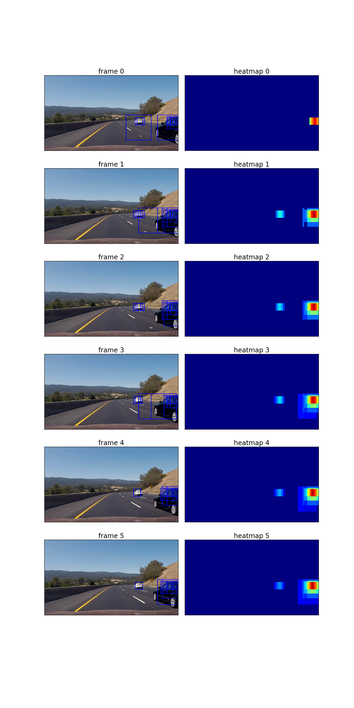Lane line positives together with false positives from rails on ht eside of the road proved very resistant to augmenting the training set unfortunately of positive detections in each frame of the video. From the positive detections I created a heatmap and then thresholded that map to identify vehicle positions.
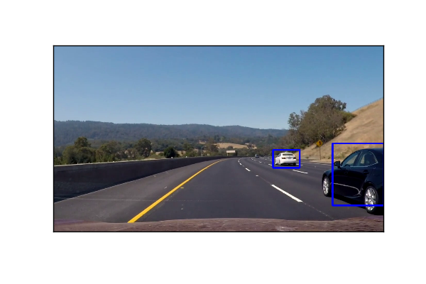
I then used scipy.ndimage.measurements.label() to identify individual blobs in the heatmap. I then assumed each blob corresponded to a vehicle. Finally I constructed bounding boxes to cover the area of each blob detected.

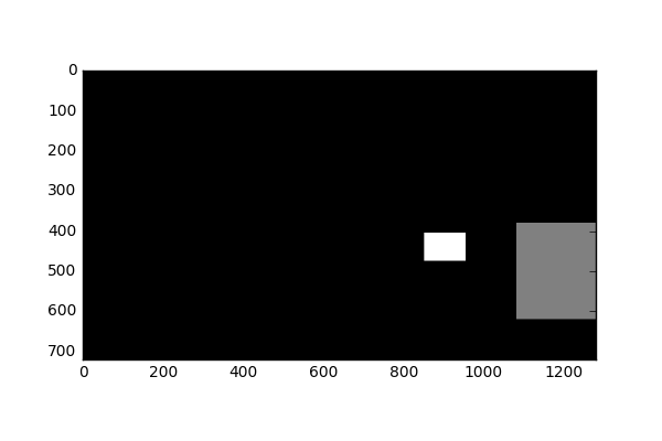
Here is an example result showing the heatmap from a series of 6 frames of video The above six frames are then integrated and thresholded. Using the output of scipy.ndimage.measurements.label() on this integrated heatmap results in an image of labels:

Finally the resulting bounding boxes are drawn onto the last frame in the series.

Comparsion to YOLO

While I was happy with the results of an SVM + HOG approach running at about 3FPS, I also wanted to check what a state of the art deep network could do. This comparison is anything but fair. We did not use the GPU at all for the SVM + HOG approach and I am shamelessly comparing apples and pears here. YOLO stands for "You only look once" and tiles an image into a modest number of squares. Each of the squares is responsible for predicting whether there is an object centered around it and if so predicting the shape of its bounding box, together with a confidence level. 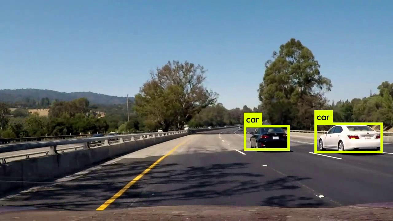For comparsion I cloned and compiled the original YOLO implementation from the darknet website. Please read more about YOLO here. I used the weights of YOLOv2 trained on the Common Objects in Context dataset (COCO) which are also available at the darknet website. Feeding in the project video on a GTX 1080 averages about 65 FPS or about 20x faster than the current SVM + HOG pipeline. Here is the result of passing the project video through YOLOv2: yolo-result.avi.

This is a very exciting result. Note that false positives are practically absent. So there is no need at all here for a heatmap, although it certainly could be used to reduce any possible false positives. I vehicle detection with YOLO type networks are an exciting direction to investigate for self-driving cars. Another direction would be to train YOLO on the Udacity training set linked to above. But these will be checked in different projects.

Discussion

Problems / issues encountered and outlook

1. I started out with a linear SVM due to its fast evaluation. Nonlinear kernels such as rbf take not only longer to train, but also much longer to evaluate. Using the linear SVM I obtained execution speeds of 3 FPS which is rather slow. However, there is ample room for improvement. At the moment the HOG features are computed for every single image which is inefficient. A way to improve speed would be to compute the HOG features only once for the entire region of interest and then select the right feature vectors, when the image is slid across.

2. The evaluation of feature vectors is currently done sequentially, but could easily be parallelized, e.g. using OpenMP. However, this would require rewriting the code in C++.

3. Some false positives still remain after heatmap filtering. This should be improvable by using more labeled data.