datadesk / Django For Data Analysis Nicar 2016
Programming Languages
Django for Data Analysis
Who are we, and what are we doing here?
So you know some SQL, or maybe done data analysis with R, but would prefer a more integrated way to explore and publish data.
In addition to making front-facing web apps, Django can also be used internally as a reporting and research tool to explore a dataset.
To do this, we'll use a publicly available dataset from the City of L.A.'s data portal on response times to complaints filed to the Department of Building and Safety. We used this data to publish a story on the varying response times to DBS complaints throughout the city, including especially slow response times on the East side of L.A.
We'll learn how to:
- Load data from a CSV into Django models.
- Create queries and views to help us analyze the data.
- Create tables and vizualizations that we can use for publication.
That's a lot of ground to cover in 60 minutes, so this will be like a cooking show. We'll walk through the steps, but the final product is mostly already baked, just waiting in the oven.
To demonstrate, here's Julia Child dancing with a turkey:

Setup
Installation
If you're on a classroom-provided computer, or have already installed the requirements, skip down to Database setup.
Otherwise, start by creating a virtual environment and clone the repo.
$ virtualenv django-for-data-analysis-nicar-2016
$ cd django-for-data-analysis-nicar-2016
$ . bin/activate
$ git clone [email protected]:datadesk/django-for-data-analysis-nicar-2016.git repo
$ cd repo
Then, install the requirements by typing or pasting the two commands below. This uses a Python data stack of NumPy, SciPy and Pandas, so it takes a loooong time to install. I highly recommend you do this before the class, if possible.
# If you're using Ubuntu, and have not installed SciPy before
# you may need to install these system libraries
$ sudo apt-get install gfortran libopenblas-dev liblapack-dev
# we have to install numpy first due to some bugs with the numpy install
$ pip install numpy==1.8.1
$ pip install -r requirements.txt
Database setup
If you're on a classroom-provided computer, a couple of commands to start. Open your terminal and type or paste:
$ workon adv_django
$ cd /data/advanced_django
Everybody now:
$ createdb django_data_analysis
$ python manage.py syncdb
This will give you a couple of prompts:
You just installed Django's auth system, which means you don't have any superusers defined.
Would you like to create one now? (yes/no):
Enter "yes", and pick a username and password you will remember. You can skip the email field.
Next, more setup to migrate the database.
$ python manage.py schemamigration building_and_safety --init
$ python manage.py migrate
Getting started: The Models
First, let's look at our models, and how they correspond to our source data CSVs. There are a couple of fields we're concerned with or need more explanation. In your text editor or browser, open up models.py and building_and_safety/data/Building_and_Safety_Customer_Service_Request__out.csv
|CSR Number|LADBS Inspection District|Address House Number|Address House Fraction Number|Address Street Direction|Address Street Name|Address Street Suffix|Address Street Suffix Direction|Address Street Zip|Date Received|Date Closed|Due Date|Case Flag|CSR Priority|GIS Parcel Identification Number (PIN)|CSR Problem Type|Area Planning Commission (APC)|Case Number Related to CSR|Response Days|Latitude/Longitude| |:---|---:|---:|---:|---:|---:|---:|---:|---:|---:|---:|---:|---:|---:|---:|---:|---:|---:|---:|---:|---:| |263018|4500|19841| |W|VENTURA|BLVD| |91367|3/1/2011||3/21/2011|N|3|174B113 358|"ISSUES REGARDING ADULT ENTERTAINMENT LOCATIONS (CLUBS, CABARETS, BOOK AND VIDEO STORES)"|South Valley|||(34.1725, -118.5653)| |265325|2142|972| |N|NORMANDIE|AVE| |90029|4/7/2011||5/5/2011|N|3|144B197 1166|FENCES WALLS AND HEDGES THAT ARE TOO HIGH|Central|||(34.08833, -118.30032)| |265779|2142|1402| |N|ALEXANDRIA|AVE| |90027|4/14/2011||5/12/2011|N|3|147B197 909|FENCES WALLS AND HEDGES THAT ARE TOO HIGH|Central|||(34.0967, -118.29815)|
- csr - This stands for customer service request ID, and can serve as our primary key.
- ladbs_inspection_district - How LADBS divides their inspectors, one per district. After reporting this out further we found that these actually change quite a bit from year-to-year.
- date_received - Date the complaint was received.
- date_closed - "Closed" is a funny term here. This is actually the date that an inspector visited the location of a complaint. In many cases this is when an inspector determines whether a complaint is valid or not. So really "closed" just means an inspector has visited a complaint.
- date_due - Arbitrary measure of time that the LADBS would like to address a complaint by. They apparently don't place a whole lot of meaning on this, and not all complaints have due dates.
- csr_priority - This is the priority level that LADBS responds to the complaints. Level 1 is often life-threatening, level 2 is quality of life issues, and level 3 is more like a nuisance.
- area_planning_commission - One of the seven different planning department areas the complaint is located in. We used this and the neighborhood level for most of our analysis.
- response_days - This should reflect the number of days it takes to respond to a complaint, however it is calculated differently for open and closed cases. So, this is a good example of why you need to understand your data. We calculated this field manually.
There are also a few fields that we're calculating at the time we load the data:
- full_address - Caching the address by concatenating the seven different address fields.
- is_closed - An easier way to find whether a case is "closed" or not.
- days_since_complaint - Our calculated "response_days" field from above. Finds the difference between the date received and the date closed.
- gt_30_days, gt_90_days, gt_180_days, more_than_one_year - Different booleans to make it easy to access cases of a certain age.
Then, let's load the complaints data using a custom management command you can see here: building_and_safety/management/commands/load_complaints.py
$ python manage.py load_complaints
The city provides two CSVs of data -- one for open cases and another for closed. This command creates a Complaint record for every row in our two csvs. Note that instead of saving every individual record as it's loaded, we use Django's bulk_create method to create them in batches of 500. This saves time because we're not hitting the database for every row in the CSV.
What are we looking at here? Exploring the data
We can use our shell to explore the data with Django's query sets.
$ python manage.py shell
Let's use this to answer a couple of basic questions about the data:
- How many complaints do we have total?
- How many are still unaddressed?
- How many complaints went more than a year before being addressed?
>>> from building_and_safety.models import Complaint
>>> complaints = Complaint.objects.all()
>>> complaints.count()
71120
>>> complaints.filter(is_closed=False).count()
4060
>>> complaints.filter(more_than_one_year=True).count()
1231
Whats happening behind the scenes?
Django's converting all of our queries to SQL, and executing them on the database. When we write code like complaints = Complaint.objects.all() Django is creating a queryset, an easy way to filter and slice our data without hitting the database. The database is only queried once we call something that evaluates the queryset, like .count().
We can see these, and it's helpful to see exactly what Django's trying to do when you're having trouble with a query.
>>> from django.db import connection
>>> print connection.queries[-1]
{u'time': u'0.028', u'sql': u'SELECT COUNT(*) FROM "building_and_safety_complaint" WHERE "building_and_safety_complaint"."more_than_one_year" = true '}
We can use this for more complicated questions too. How are the complaints older than one year distributed throughout the planning commissions? Are some worse than others?
>>> from django.db.models import Count
>>> complaints.filter(more_than_one_year=True).values('area_planning_commission').annotate(count=Count("csr")).order_by('-count')
[{
    'count': 618,
    'area_planning_commission': u'East Los Angeles'
}, {
    'count': 394,
    'area_planning_commission': u'Central'
}, {
    'count': 86,
    'area_planning_commission': u'West Los Angeles'
}, {
    'count': 60,
    'area_planning_commission': u'South Valley'
}, {
    'count': 56,
    'area_planning_commission': u'South Los Angeles'
}, {
    'count': 8,
    'area_planning_commission': u'North Valley'
}, {
    'count': 7,
    'area_planning_commission': u''
}, {
    'count': 2,
    'area_planning_commission': u'Harbor'
}]
Now we're on to something.
The views: A first look
One advantage of using Django is that all of our data manipulation can be stored in views, and the output displayed in HTML templates.
We've already created a few views that summarize the data, so let's take a look.
Exit the Python interpreter, if you still have it running, by pressing CTRL-D, and start the Django server.
$ python manage.py runserver
Validating models...

0 errors found
February 20, 2016 - 16:40:36
Django version 1.6.5, using settings 'project.settings'
Starting development server at http://0.0.0.0:8000/
Quit the server with CONTROL-C.
In the spirit of a cooking show, let's cheat. Let's see what we're going to get first, and then look at how we get it. In your web browser, go to http://localhost:8000/complaint_analysis.
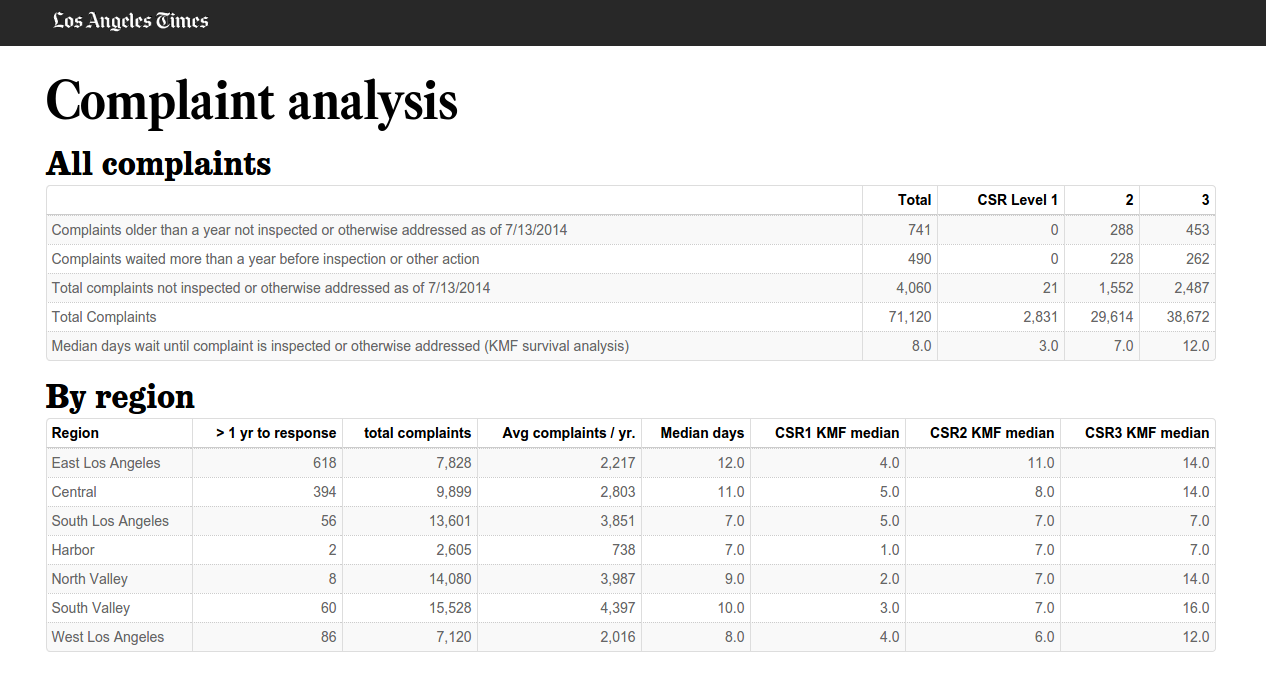
Here is a table with some basic information about our complaints. How many have been addressed, how many are still open, and how many have hung around for a really long time.
In the second table, we also break this down by area planning commissions - areas used by the L.A. Department of City Planning to divide up the city.
A primer on survival analysis
For our analysis, we want to get the median time it takes to close a complaint. Simply calculating the median based on complaints that are already closed leaves out all of the complaints that are still open -- including those that have lingered in the system unaddressed for more than a year.
Using a statistical method called survival analysis can help us account for complaints still open, and give us a more accurate closure time.
Survival analysis was created for use by actuaries and medical professionals to measure lifespans of individuals. It can be used to analyze not only literal births and deaths, but also any instance where a "birth" or "death" can be observed. In this case, a "birth" is the opening of a complaint, and "death" is that complaint being visited and marked as "closed."
The excellent Lifelines documentation has another example of survival analysis looking at the tenure of world leaders, where the "birth" is the start of their time in office and the "death" is their departure.
Another example was performed by Times database editor Doug Smith and data analyst Brian Kim in finding that youths in California's privatized foster care remained in the foster system 11% longer than those in other types of homes — 378 days compared to 341 days.
There are libraries in R that can do this as well, (see survival and KMsurv,) but using a Python library keeps this all in the same development stack.
Diving into the views
Open up the views.py file in your text editor, and look at the ComplaintAnalysis view.
There's a lot going on here. We know there were more complaints open after a year in East L.A. than other parts of the city. But is this because they receive more complaints in general? Are some types of complaints addressed more quickly than others?
To find the median time to address a complaint, we use survival analaysis. Let's take apart this view:
class ComplaintAnalysis(TemplateView):
    # The HTML template we're going to use, found in the /templates directory
    template_name = "complaint_analysis.html"
This defines the ComplaintAnalysis as a template view, and sets the HTML template that we're going to build with the data generated from the view. You can either open complaint_analysis.html in your text editor, or follow the link here.
# Quick notation to access all complaints
complaints = Complaint.objects.all()

# Quick means of accessing both open and closed cases
open_cases = complaints.filter(is_closed=False)
closed_cases = complaints.filter(is_closed=True)

# Overall complaints not addressed within a year
over_one_year = complaints.filter(more_than_one_year=True)
open_over_one_year = over_one_year.filter(is_closed=False)
closed_over_one_year = over_one_year.filter(is_closed=True)
We then split our complaints into four groups: open, closed, open over a year, and closed over a year. We'll use these throughout the rest of the view.
# total counts of cases, all priority levels
total_count = complaints.all().count()
total_by_csr = get_counts_by_csr(complaints)

# Counts of open cases, all priority levels
open_cases_count = open_cases.count()
open_by_csr = get_counts_by_csr(open_cases)

# Counts of cases that have been open fore more than a year, all priority levels
open_over_one_year_count = open_over_one_year.count()
open_over_one_year_by_csr = get_counts_by_csr(open_over_one_year)

# Counts of cases that were closed, but have been open for more than a year, all priority levels.
closed_over_one_year_count = closed_over_one_year.count()
closed_over_one_year_by_csr = get_counts_by_csr(closed_over_one_year)
We use a helper function here to get counts of complaints for each priority level:
def get_counts_by_csr(qs):
    counts = {}
    counts["csr1"] = qs.filter(csr_priority="1").count()
    counts["csr2"] = qs.filter(csr_priority="2").count()
    counts["csr3"] = qs.filter(csr_priority="3").count()
    return counts
This function takes a queryset, and returns a dictionary of counts for each CSR. This is the programming adage of DRY, we're not repeating the same code many different times in our view.
To calculate the response times for different priority levels of complaints, we use the Kaplan-Meier fit from our survival analysis library. It will return us a median wait time, and establish a closure rate for accounts for complaints that are still open.
all_complaints = Complaint.objects.exclude(days_since_complaint__lt=0)
kmf_fit = get_kmf_fit(all_complaints)
median_wait_time_kmf = get_kmf_median(kmf_fit)
Let's take a quick look at the functions get_kmf_fit() and get_kmf_median().
# Get the average wait time using a Kaplan-Meier Survival analysis estimate
# Make arrays of the days since complaint, and whether a case is 'closed'
# this creates the observations, and whether a "death" has been observed
def get_kmf_fit(qs):
    t = qs.values_list('days_since_complaint', flat=True)
    c = qs.values_list('is_closed', flat=True)
    kmf = KaplanMeierFitter()
    kmf.fit(t, event_observed=c)
    return kmf


# Return the mean of our KMF curve
def get_kmf_median(kmf):
    return kmf.median_
This function makes two lists: one of the count of days since a complaint was created and another of whether the complaint has been closed. Those lists are then fitted to a Kaplan-Meier curve, and the function returns the kmf object. get_kmf_median simply returns the median_ value of that object.
We use this method to find the median response time to all complaints, as well as the response time for priority level 1, 2 and 3 complaints.
Since it seems like response times are slower in the eastern parts of the city, let's break it down further. We make a list of the seven different planning commission areas, and then store the results in a dictionary.
region_names = ['Central','East Los Angeles','Harbor','North Valley','South Los Angeles','South Valley','West Los Angeles']
regions = {}
Then, we iterate over those region names, creating a queryset and aggregate counts for each area.
# Iterate over each name in our region_names list
for region in region_names:
    # Filter for complaints in each region
    qs = complaints.filter(area_planning_commission=region, days_since_complaint__gte=0)
    # create a data dictionary for the region
    regions[region] = {}
    # get a count of how many complaints total are in the queryset
    regions[region]['total'] = qs.count()
Let's also find the volume of complaints each area receives in a year.
regions[region]['avg_complaints_per_year'] = get_avg_complaints_filed_per_year(region)
Let's use survival analysis to find the median response time for each priority level of complaint. This is basically the same thing we did above, but for a smaller queryset of complaints confined to each planning commission area.
# Separate the complaints into querysets of their respective priority levels
region_csr1 = qs.filter(csr_priority="1")
region_csr2 = qs.filter(csr_priority="2")
region_csr3 = qs.filter(csr_priority="3")

# Find the KMF fit for all complaints in the area and by each priority level
regional_kmf_fit = get_kmf_fit(qs)
regional_kmf_fit_csr1 = get_kmf_fit(region_csr1)
regional_kmf_fit_csr2 = get_kmf_fit(region_csr2)
regional_kmf_fit_csr3 = get_kmf_fit(region_csr3)

# Get the median value from the KMF fit.
regions[region]['median_wait_kmf'] = get_kmf_median(regional_kmf_fit)
regions[region]['median_wait_kmf_csr1'] = get_kmf_median(regional_kmf_fit_csr1)
regions[region]['median_wait_kmf_csr2'] = get_kmf_median(regional_kmf_fit_csr2)
regions[region]['median_wait_kmf_csr3'] = get_kmf_median(regional_kmf_fit_csr3)
Last, we also find the number of complants greater than a year in each area.
regions[region]['gt_year'] = qs.filter(more_than_one_year=True).count()
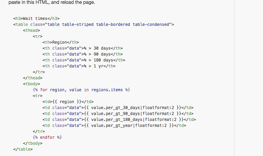
We have complaints over a year, but where are the response times breaking down? Let's also find the number of complaints older than 30, 90, 180 days and one year, and use latimes-calculate to find the what percentage of the total complaints fall in these categories.
Now let's take a look at this in the template. Open up complaint_analysis.html in your text editor and in your browser at http://localhost:8000/complaint_analysis/.
This page is two HTML tables. Notice the values wrapped in {{foo}} curly brackets. These are the variables from our view that get fed into the template. We can use them in a number of ways, here, we simply feed them in as table values.
You'll also see values like |intcomma or |floatformat:1. These are brought in from the humanize set of template filters, that make numbers easier to read and understand. See the load statement in line 2, {% load humanize toolbox_tags %} that brings in this set of filters.
Go ahead and remove one of the floatformat filters and reload the page. Rounding is good!
We have summary data for all complaints, and for complants broken down by region. Let's use the new variables we created in the view on what percentage of complaints took longer than 30, 90 and 180 days to build a new table.
Below the regional breakdown table, but before the {% endblock %} tag (around line 95), type or paste in this HTML, and reload the page.
<h3>Wait times</h3>
<table class="table table-striped table-bordered table-condensed">
    <thead>
        <tr>
            <th>Region</th>
            <th class="data">% > 30 days</th>
            <th class="data">% > 90 days</th>
            <th class="data">% > 180 days</th>
            <th class="data">% > 1 yr</th>
        </tr>
    </thead>
    <tbody>
        {% for region, value in regions.items %}
        <tr>
            <td>{{ region }}</td>
            <td class="data">{{ value.per_gt_30_days|floatformat:2 }}</td>
            <td class="data">{{ value.per_gt_90_days|floatformat:2 }}</td>
            <td class="data">{{ value.per_gt_180_days|floatformat:2 }}</td>
            <td class="data">{{ value.per_gt_year|floatformat:2 }}</td>
        </tr>
        {% endfor %}
    </tbody>
</table>
Using this method you can analyze and present your data in a number of ways that can help you find and understand the story.
Visualizing the data: Let's make a map
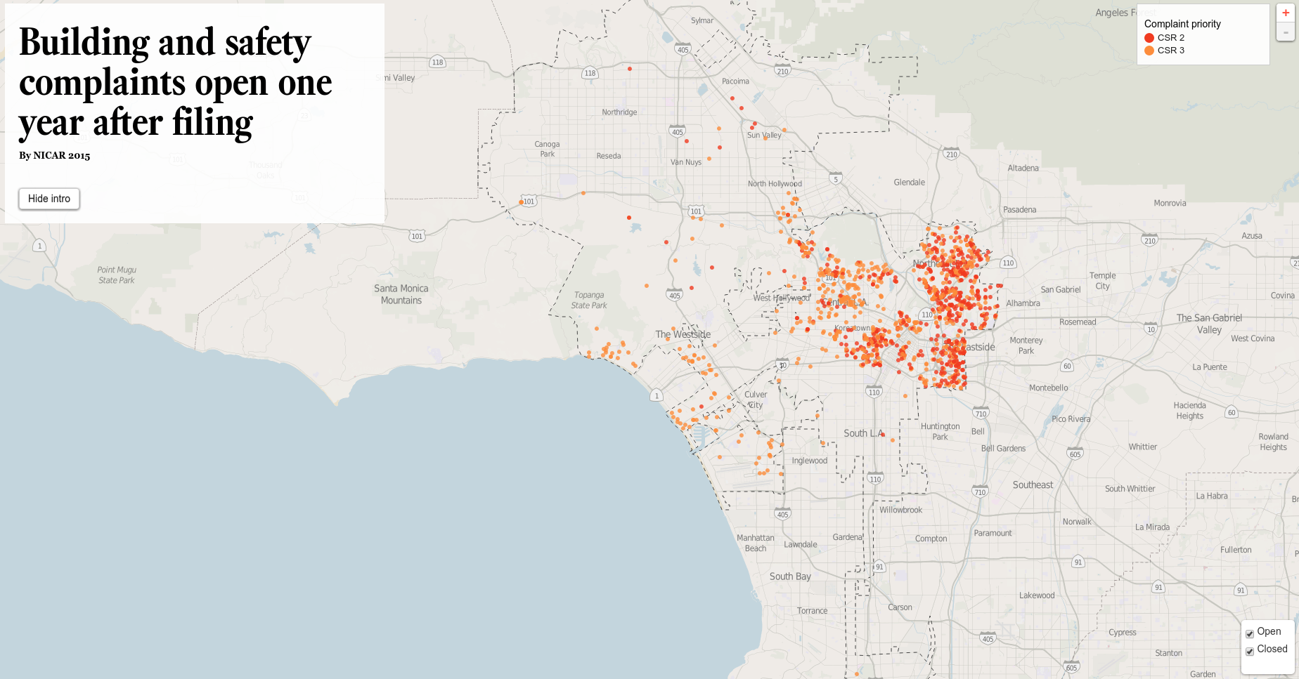
Take a look at the view ComplaintsMap.
What's happening here? It doesn't look like anything's in the view, right? Let's take a look at the template. Open up templates/complaints_map.html
This template calls two other views through a $.getJSON() call - open_complaints_json and closed_complaints_json.
These two views are essentially the same, pulling in all geocoded complaints that waited more than a year for a response, except one pulls in closed and one pulls in open complaints.
Both use a method on the Complaint model to export relevant fields of the model to a GeoJSON object.
features = [complaint.as_geojson_dict() for complaint in complaints]
This refers back the as_geojson_dict() method on the Complaint model. This method takes properties from the model and returns them in a geojson dict format:
def as_geojson_dict(self):
  """
  Method to return each feature in the DB as a geojson object.
  """
  as_dict = {
      "type": "Feature",
      "geometry": {
          "type": "Point",
          "coordinates": [
              float(self.lon),
              float(self.lat)
          ]
      },
      "properties": {
          "address": self.full_address,
          "csr": self.csr,
          "date": dateformat.format(self.date_received, 'F j, Y'),
          "closed": self.get_closed_date(),
          "type": self.csr_problem_type,
          "priority": self.csr_priority
      }
  }
  return as_dict
We get this dict for each item in the queryset, and then form them into a geojson object that is returned when we request the view.
objects = {
    'type': "FeatureCollection",
    'features': features
}
response = json.dumps(objects)
return HttpResponse(response, content_type='text/json')
Try this out - go to http://localhost:8000/api/complaints.json. It loads a GeoJSON object! All those rows in the database are automatically generated in GeoJSON format.
Load the URL http://localhost:8000/complaints-map/. It should load a map in your browser.
What is this map loading in? What's it showing us? How does this demonstrate the flexibility of using a Django backend instead of exporting our results from SQL or another database format?
Take a look at the views for open_complaints_json and closed_complaints_json - we're filtering for all complaints older than a year, and excluding any without geocoded lat/lon points.
Say, later in the editing process, we want to export only complaints older than 180 days, instead of a year. In Django, this is easy:
complaints = Complaint.objects\
        .filter(is_closed=True, gt_180_days=True).exclude(lat=None, lon=None)
Go ahead and change that in the open_complaints_json and closed_complaints_json views now, and reload the map. You'll see the changes instantly. Instead of having to go back to the database, re-enter our SQL, and re-export our files, Django takes care of all of that for you.
Later, if we decide not to include the closed complaints, for example, we can simply remove that call in the template.
You can also change the information that's fed into the GeoJSON object. Maybe we want to add the area planning commission, and the number of days since the complaint was filed?
Let's add this in line 148 of models.py
"properties": {
    "address": self.full_address,
    "csr": self.csr,
    "date": dateformat.format(self.date_received, 'F j, Y'),
    "closed": self.get_closed_date(),
    "type": self.csr_problem_type,
    "priority": self.csr_priority,
    "apc": self.area_planning_commission,
    "days_since_complaint": self.days_since_complaint
}
And we'll modify our leaflet tooltip to pull in this information in complaints_map.html. On line 166, we feed those properties to our underscore template.:
var context = {
    address: props["address"],
    csr: props["csr"],
    date: props["date"],
    closed_date: props["closed"],
    priority: priority,
    problem: props["type"],
    apc: props["apc"],
    days_since_complaint: props["days_since_complaint"]
};
And update the underscore template on line 74.
<script type="text/template" id="tooltip-template">
    <h4><a href="/complaint/<%= csr %>/"><%= address %></a></h4>
    <p>CSR number <a href="/complaint/<%= csr %>/"><%= csr %></a></p>
    <p>Received <%= date %></p>
    <% if (closed_date !== null) { %><p>Closed <%= closed_date %></p><% } %>
    <p>Priority <%= priority %> complaint</p>
    <p><%= problem %></p>
    <p><%= days_since_complaint %> days since complaint was filed.</p>
    <p><%= apc %> planning commission</p>
</script>
So you can pretty quickly add or remove properties from your data and your templates.
Pitfalls of Django
Like anything, there are a few disadvantages to using Django as a reporting framework.
It's a lot of up-front work.
- There's no doubt that setting up a Django project takes a lot of time to get started and running. Models and loader scripts take planning, and we're all on a constant time crunch. And not every project merits this, sometimes you can get the results you need with a few quick pivot tables or R scripts. But the saved time in the analysis and publication phases make it well worth the input for me.
With huge databases (and a slow computer) the queries can take forever
- This can be a problem with large datasets, but there are a few solutions. Caching is one. Django has a number of built-in caching options to help out with this. Another possible option is to bake out any visualizations that will be used for publication. Django-bakery can help with this.
Check, check, check your data
- Because it's so easy to swap things around, or filter a queryset, it's easy to think you're looking at one thing, but you're actually looking at another. What if we had filtered for complaints over 90 days, when we thought we were looking at 180?
- Fortunately, since everything is written down and traceable in the views, it's fairly easy to spot and correct possible errors before publication.
What can we do from here?
We skipped it for this lesson, but in the original story, we used GeoDjango and a GIS-enabled database to allow for geospatial queries on the data - This allowed us to relate complaints to L.A. Times Neighborhoods shapes, and to census tracts and LADBS inspection districts.
Using GeoDjango, you can also set a buffer around a point, which is what LAT Alum Ken Schwencke did for this piece analyzing homicides in the unincorporated neighborhood of Westmont and along a two-mile stretch of Vermont Ave. called "Death Alley."