rlguy / Gridfluidsim3d
Projects that are alternatives of or similar to Gridfluidsim3d
GridFluidSim3d
This program is an implementation of a PIC/FLIP liquid fluid simulation written in C++11 based on methods described in Robert Bridson's "Fluid Simulation for Computer Graphics" textbook. The fluid simulation program outputs the surface of the fluid as a sequence of triangle meshes stored in the Stanford .PLY file format which can then be imported into your renderer of choice.
Visit http://rlguy.com/gridfluidsim/ for more information about the program.
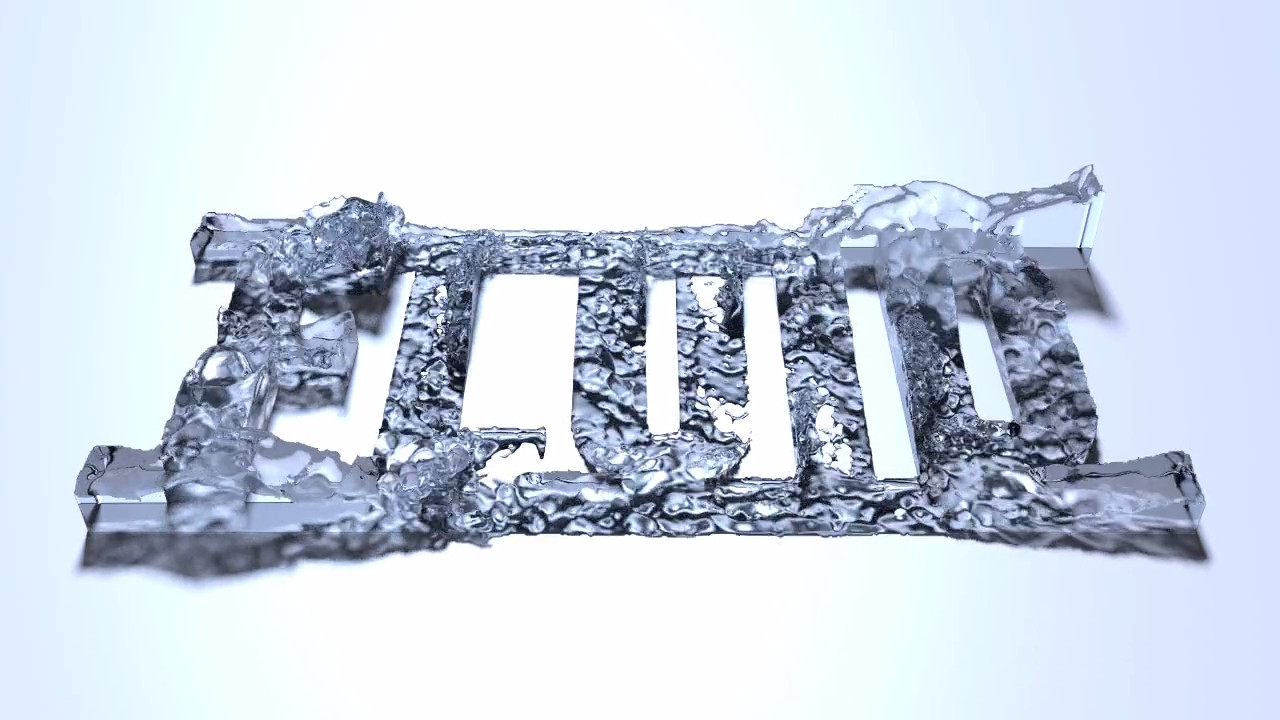
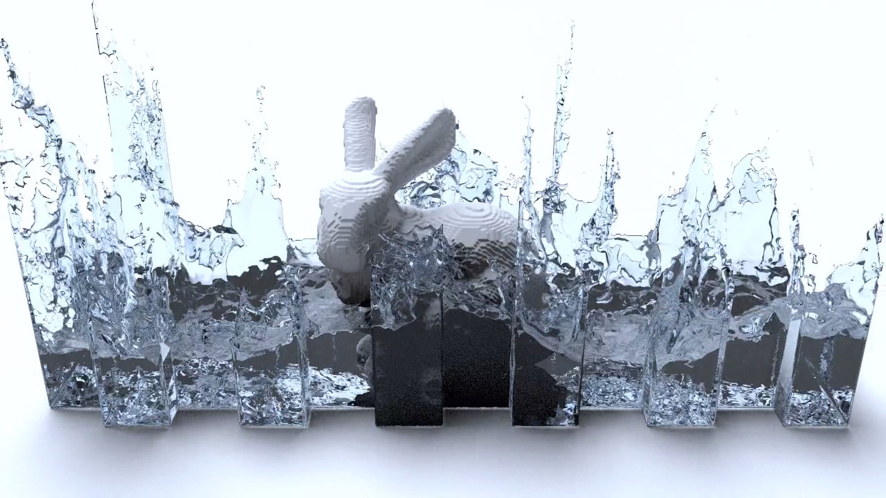
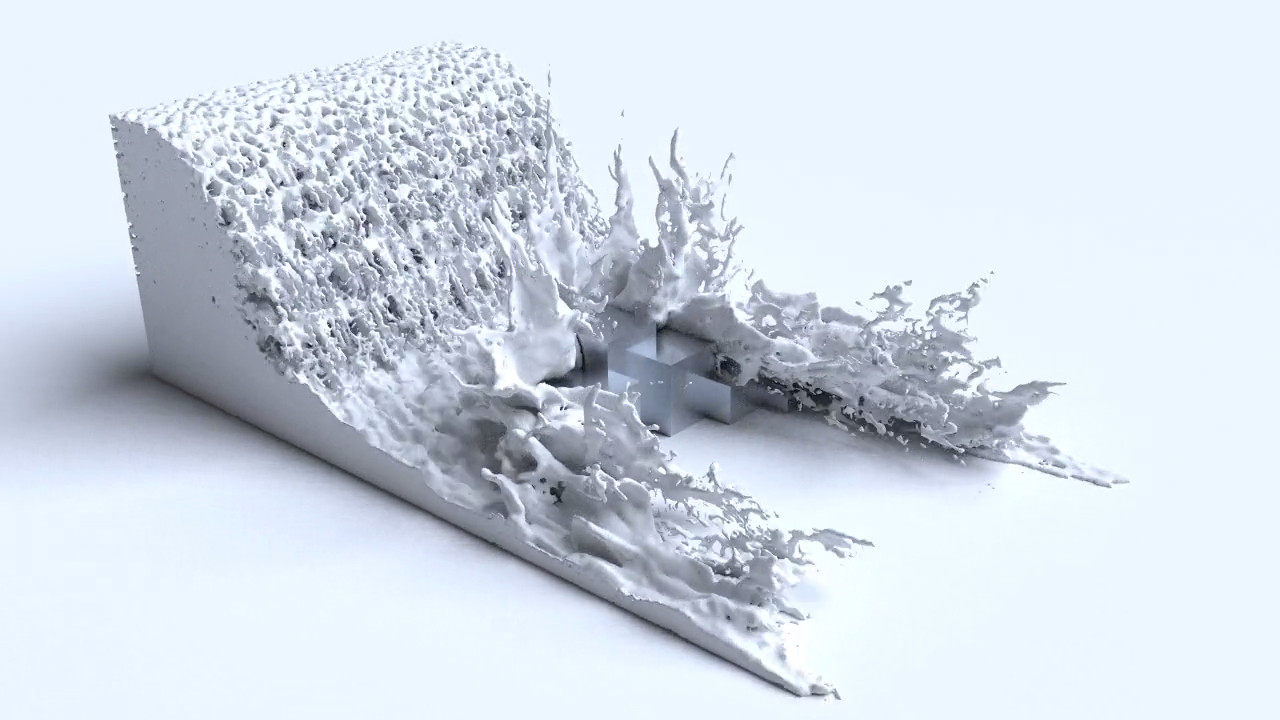
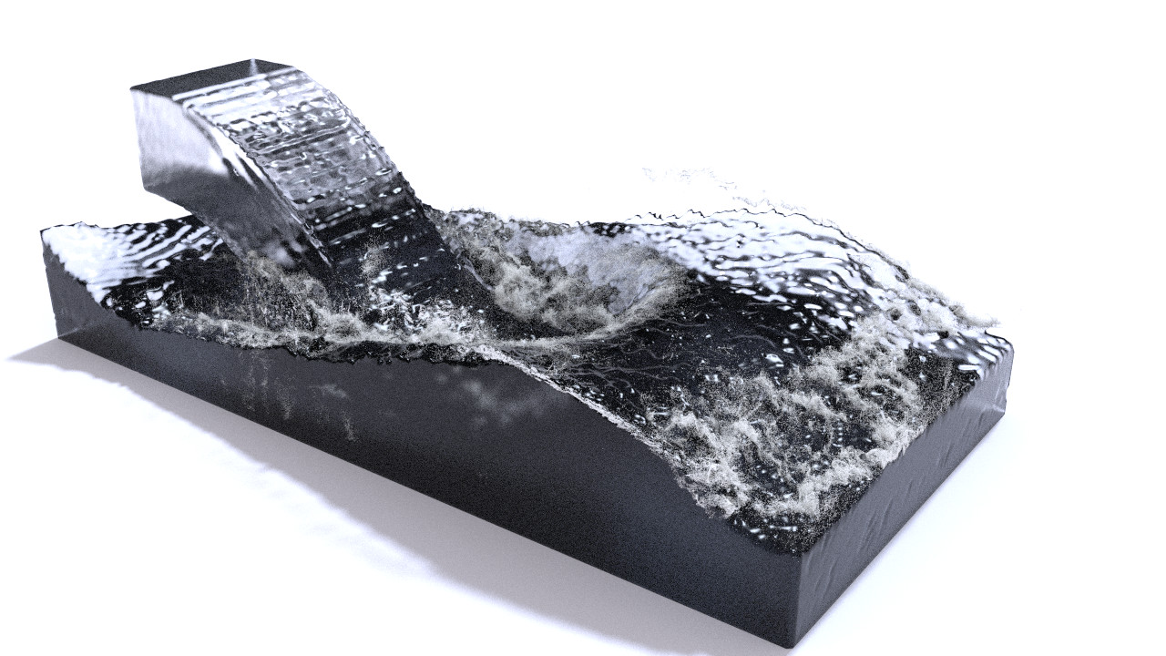
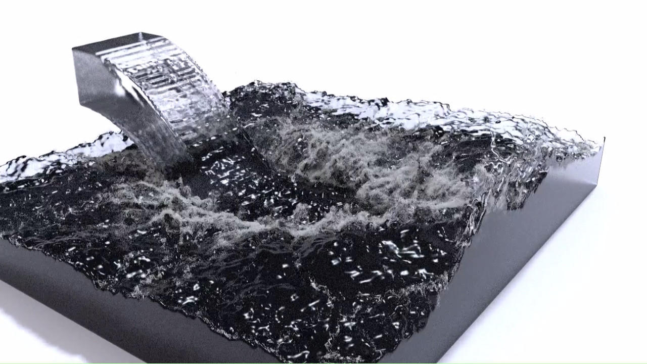
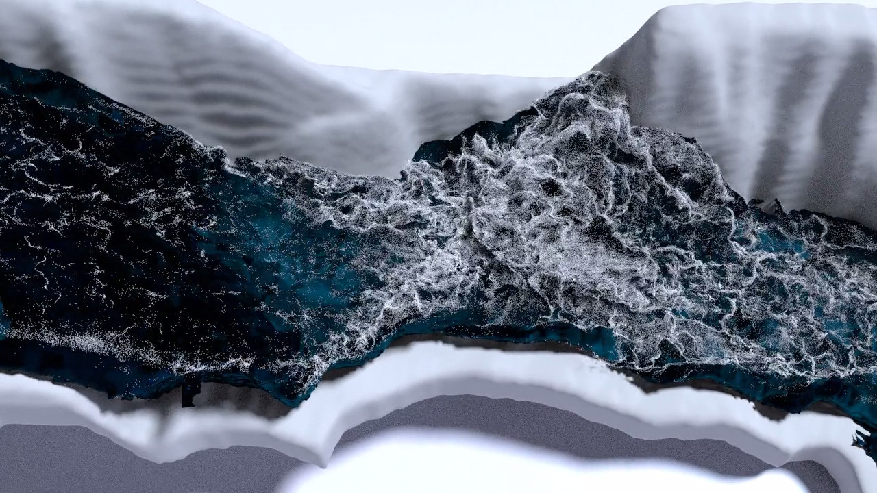
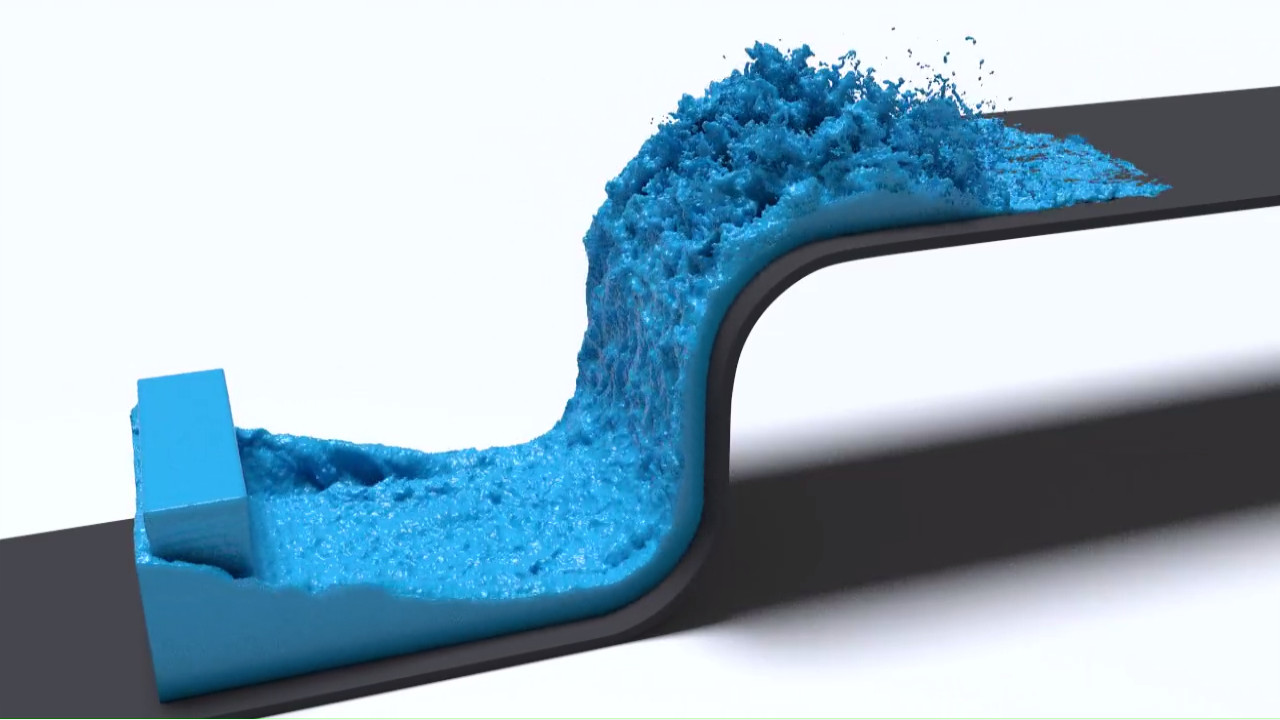
Gallery
The following screencaps are of animations that were simulated within the program and rendered using Blender. Animations created with the fluid simulation program can be viewed on YouTube.


Features
Below is a list of features implemented in the simulator.
- Isotropic and anisotropic particle to mesh conversion
- Spray, bubble, and foam particle simulation
- 'LEGO' brick surface reconstruction
- Save and load state of a simulation
- GPU accelerated fourth-order Runge-Kutta integration using OpenCL
- GPU accelerated velocity advection using OpenCL
- Python bindings
Dependencies
There are three dependencies that are required to build this program:
- OpenCL headers (can be found at khronos.org)
- An OpenCL SDK specific to your GPU vender (AMD, NVIDIA, Intel, etc.)
- A compiler that supports C++11
Installation
This program uses the CMake utility to generate the appropriate solution, project, or Makefiles for your system. The following commands can be executed in the root directory of the project to generate a build system for your machine:
mkdir build && cd build
cmake ..
The first line creates a new directory named build and changes the working directory to the newly created build directory. The second line runs the CMake utility and passes it the parent directory which contains the CMakeLists.txt file.
The type of build system generated by CMake can be specified with the -G [generator] parameter. For example:
cmake .. -G "MinGW Makefiles"
will generate Makefiles for the MinGW compiler which can then be built using the GNU Make utility with the command make. A list of CMake generators can be found here.
Once successfully built, the program will be located in the build/fluidsim/ directory with the following directory structure:
fluidsim
│   fluidsim.a      - Runs program configured in main.cpp
│
└───output          - Stores data output by the simulation program
│   └───bakefiles       - meshes
│   └───logs            - logfiles
│   └───savestates      - simulation save states
│   └───temp            - temporary files created by the simulation program
│
└───pyfluid         - The pyfluid Python package
    └───examples        - pyfluid example usage
    └───lib             - C++ library files
Configuring the Fluid Simulator
The fluid simulator can be configured by manipulating a FluidSimulation object in the function main() located in the file src/main.cpp. After building the project, the fluid simulation exectuable will be located in the fluidsim/ directory. Example configurations are located in the src/examples/cpp/ directory. Some documentation on the public methods for the FluidSimulation class is provided in the fluidsimulation.h header.
A fluid simulation can also be configured and run within a Python script by importing the pyfluid package, which will be located in the fluidsim/ directory after building the project. Example scripts are located in the src/examples/python/ directory.
The following two sections will demonstrate how to program a simple "Hello World" simulation using either C++ or Python.
Hello World (C++)
This is a very basic example of how to use the FluidSimulation class to run a simulation. The simulation in this example will drop a ball of fluid in the center of a cube shaped fluid domain. This example is relatively quick to compute and can be used to test if the simulation program is running correctly.
The fluid simulator performs its computations on a 3D grid, and because of this the simulation domain is shaped like a rectangular prism. The FluidSimulation class can be initialized with four parameters: the number of grid cells in each direction x, y, and z, and the width of a grid cell.
int xsize = 32;
int ysize = 32;
int zsize = 32;
double cellsize = 0.25;
FluidSimulation fluidsim(xsize, ysize, zsize, cellsize);
We want to add a ball of fluid to the center of the fluid domain, so we will need to get the dimensions of the domain by calling getSimulationDimensions and passing it pointers to store the width, height, and depth values. Alternatively, the dimensions can be calculated by multiplying the cell width by the corresponding number of cells in a direction (e.g. width = dx*isize).
double width, height, depth;
fluidsim.getSimulationDimensions(&width, &height, &depth);
Now that we have the dimensions of the simulation domain, we can calculate the center, and add a ball of fluid by calling addImplicitFluidPoint which takes the x, y, and z position and radius as parameters.
double centerx = width / 2;
double centery = height / 2;
double centerz = depth / 2;
double radius = 6.0;
fluidsim.addImplicitFluidPoint(centerx, centery, centerz, radius);
An important note to make about addImplicitFluidPoint is that it will not add a sphere with the specified radius, it will add a sphere with half of the specified radius. An implicit fluid point is represented as a field of values on the simulation grid. The strength of the field values are 1 at the point center and falls off towards 0 as distance from the point increases. When the simulation is initialized, fluid particles will be created in regions where the field values are greater than 0.5. This means that if you add a fluid point with a radius of 6.0, the ball of fluid in the simulation will actually be of radius 3.0 since field values will be less than 0.5 at a distance greater than half of the specified radius.
The FluidSimulation object now has a domain containing some fluid, but the current simulation will not be very interesting as there are no forces acting upon the fluid. We can add the force of gravity by making a call to addBodyForce which takes three values representing a force vector as parameters. We will set the force of gravity to point downwards with a value of 25.0.
double gx = 0.0;
double gy = -25.0;
double gz = 0.0;
fluidsim.addBodyForce(gx, gy, gz);
Now we have a simulation domain with some fluid, and a force acting on the fluid. Before we run the simulation, a call to initialize must be made. Note that any calls to addImplicitFluidPoint must be made before initialize is called.
fluidsim.initialize();
We will now run the simulation for a total of 30 animation frames at a rate of 30 frames per second by repeatedly making calls to the update function. The update function advances the state of the simulation by a specified period of time. To update the simulation at a rate of 30 frames per second, each call to update will need to be supplied with a time value of 1.0/30.0. Each call to update will generate a triangle mesh that represents the fluid surface. The mesh files will be saved in the output/bakefiles/ directory as a numbered sequence of files stored in the Stanford .PLY file format.
double timestep = 1.0 / 30.0;
int numframes = 30;
for (int i = 0; i < numframes; i++) {
    fluidsim.update(timestep);
}
As this loop runs, the program should output simulation stats and timing metrics to the terminal. After the loop completes, the output/bakefiles/ directory should contain 30 .PLY triangle meshes numbered in sequence from 0 to 29: 000000.ply, 000001.ply, 000002.ply, ..., 000028.ply, 000029.ply.
If you open the 000029.ply mesh file in a 3D modelling package such as Blender, the mesh should look similar to this image.
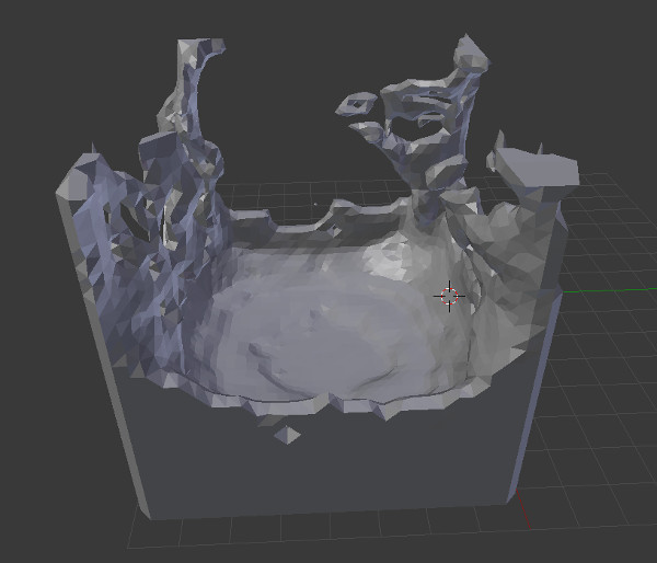
The fluid simulation in this example is quick to compute, but of low quality due to the low resolution of the simulation grid. The quality of this simulation can be improved by increasing the simulation dimensions while decreasing the cell size. For example, try simulating on a grid of resolution 64 x 64 x 64 with a cell size of 0.125, or even better, on a grid of resolution 128 x 128 x 128 with a cell size of 0.0625.
Hello World (Python)
The following Python script will run the equivalent simulation described in the previous section.
from pyfluid import FluidSimulation

fluidsim = FluidSimulation(32, 32, 32, 0.25)

width, height, depth = fluidsim.get_simulation_dimensions()
fluidsim.add_implicit_fluid_point(width / 2, height / 2, depth / 2, 6.0)
fluidsim.add_body_force(0.0, -25.0, 0.0)
fluidsim.initialize();

for i in range(30):
    fluidsim.update(1.0 / 30)