One Cycle Learning Rate Policy for Keras

Implementation of One-Cycle Learning rate policy from the papers by Leslie N. Smith.

• A disciplined approach to neural network hyper-parameters: Part 1 -- learning rate, batch size, momentum, and weight decay
• Super-Convergence: Very Fast Training of Residual Networks Using Large Learning Rates

Contains two Keras callbacks, LRFinder and OneCycleLR which are ported from the PyTorch Fast.ai library.

What is One Cycle Learning Rate

It is the combination of gradually increasing learning rate, and optionally, gradually decreasing the momentum during the first half of the cycle, then gradually decreasing the learning rate and optionally increasing the momentum during the latter half of the cycle.

Finally, in a certain percentage of the end of the cycle, the learning rate is sharply reduced every epoch.

The Learning rate schedule is visualized as :

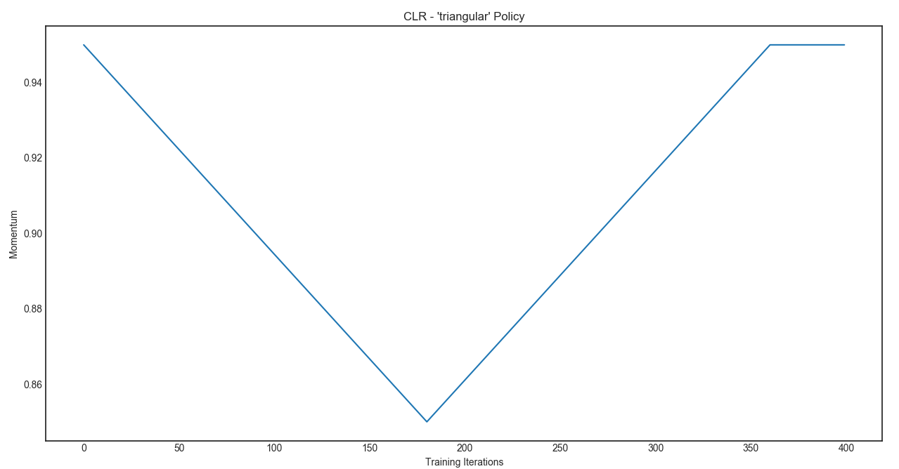
The Optional Momentum schedule is visualized as :

Usage

Finding a good learning rate

Use LRFinder to obtain a loss plot, and visually inspect it to determine the initial loss plot. Provided below is an example, used for the MiniMobileNetV2 model.

An example script has been provided in find_lr_schedule.py inside the models/mobilenet/.

Essentially,

from clr import LRFinder

lr_callback = LRFinder(num_samples, batch_size,
                       minimum_lr, maximum_lr,
                       # validation_data=(X_val, Y_val),
                       lr_scale='exp', save_dir='path/to/save/directory')

# Ensure that number of epochs = 1 when calling fit()
model.fit(X, Y, epochs=1, batch_size=batch_size, callbacks=[lr_callback])

The above callback does a few things.

• Must supply number of samples in the dataset (here, 50k from CIFAR 10) and the batch size that will be used during training.
• lr_scale is set to exp - useful when searching over a large range of learning rates. Set to linear to search a smaller space.
• save_dir - Automatic saving of the results of LRFinder on some directory path specified. This is highly encouraged.
• validation_data - provide the validation data as a tuple to use that for the loss plot instead of the training batch loss. Since the validation dataset can be very large, we will randomly sample k batches (k * batch_size) from the validation set to provide quick estimate of the validation loss. The default value of k can be changed by changing validation_sample_rate

Note : When using this, be careful about setting the learning rate, momentum and weight decay schedule. The loss plots will be more erratic due to the sampling of the validation set.

NOTE 2 :

• It is faster to get the learning rate without using validation_data, and then find the weight decay and momentum based on that learning rate while using validation_data.
• You can also use LRFinder to find the optimal weight decay and momentum values using the examples find_momentum_schedule.py and find_weight_decay_schedule.py inside models/mobilenet/ folder.

To visualize the plot, there are two ways -

• Use lr_callback.plot_schedule() after the fit() call. This uses the current training session results.
• Use class method LRFinder.plot_schedule_from_dir('path/to/save/directory') to visualize the plot separately from the training session. This only works if you used the save_dir argument to save the results of the search to some location.

Finding the optimal Momentum

Use the find_momentum_schedule.py script inside models/mobilenet/ for an example.

Some notes :

• Use a grid search over a few possible momentum values, such as [0.8, 0.85, 0.9, 0.95, 0.99]. Use linear as the lr_scale argument value.

• Set the momentum value manually to the SGD optimizer before compiling the model.

• Plot the curve at the end and visually see which momentum value yields the least noisy / lowest losses overall on the plot. The absolute value of the loss plot is not very important as much as the curve.

• It is better to supply the validation_data here.

• The plot will be very noisy, so if you wish, can use a larger value of loss_smoothing_beta (such as 0.99 or 0.995)

• The actual curve values doesnt matter as much as what is overall curve movement. Choose the value which is more steady and tries to get the lowest value even at large learning rates.

Finding the optimal Weight Decay

Use the find_weight_decay_schedule.py script inside models/mobilenet/ for an example

Some notes :

• Use a grid search over a few weight decay values, such as [1e-3, 1e-4, 1e-5, 1e-6, 1e-7]. Call this "coarse search" and use linear for the lr_scale argument.

• Use a grid search over a select few weight decay values, such as [3e-7, 1e-7, 3e-6]. Call this "fine search" and use linear scale for the lr_scale argument.

• Set the weight decay value manually to the model when building the model.

• Plot the curve at the end and visually see which weight decay value yields the least noisy / lowest losses overall on the plot. The absolute value of the loss plot is not very important as much as the curve.

• It is better to supply the validation_data here.

• The plot will be very noisy, so if you wish, can use a larger value of loss_smoothing_beta (such as 0.99 or 0.995)

• The actual curve values doesnt matter as much as what is overall curve movement. Choose the value which is more steady and tries to get the lowest value even at large learning rates.

Interpreting the plot

Learning Rate

Consider the above plot from using the LRFinder on the MiniMobileNetV2 model. In particular, there are a few regions above that we need to carefully interpret.

Note : The values are in log 10 scale (since exp was used for lr_scale) ; All values discussed will be based on the x-axis (learning rate) :

• After the -1.5 point on the graph, the loss becomes erratic
• After the 0.5 point on the graph, the loss is noisy but doesn't decrease any further.
• -1.7 is the last relatively smooth portion before the -1.5 region. To be safe, we can choose to move a little more to the left, closer to -1.8, but this will reduce the performance.
• It is usually important to visualize the first 2-3 epochs of OneCycleLR training with values close to these edges to determine which is the best.

Momentum

Using the above learning rate, use this information to next calculate the optimal momentum (find_momentum_schedule.py)

See the notes in the Finding the optimal momentum section on how to interpret the plot.

Weight Decay

Similarly, it is possible to use the above learning rate and momentum values to calculate the optimal weight decay (find_weight_decay_schedule.py).

Note : Due to large learning rates acting as a strong regularizer, other regularization techniques like weight decay and dropout should be decreased significantly to properly train the model.

It is best to search a range of regularization strength between 1e-3 to 1e-7 first, and then fine-search the region that provided the best overall plot.

See the notes in the Finding the optimal weight decay section on how to interpret the plot.

Training with OneCycleLR

Once we find the maximum learning rate, we can then move onto using the OneCycleLR callback with SGD to train our model.

from clr import OneCycleLR

lr_manager = OneCycleLR(num_samples, num_epoch, batch_size, max_lr
                        end_percentage=0.1, scale_percentage=None,
                        maximum_momentum=0.95, minimum_momentum=0.85)
                        
model.fit(X, Y, epochs=EPOCHS, batch_size=batch_size, callbacks=[model_checkpoint, lr_manager], 
          ...)

There are many parameters, but a few of the important ones :

• Must provide a lot of training information - number of samples, number of epochs, batch size and max learning rate
• end_percentage is used to determine what percentage of the training epochs will be used for steep reduction in the learning rate. At its miminum, the lowest learning rate will be calculated as 1/1000th of the max_lr provided.
• scale_percentage is a confusing parameter. It dictates the scaling factor of the learning rate in the second half of the training cycle. It is best to test this out visually using the plot_clr.py script to ensure there are no mistakes. Leaving it as None defaults to using the same percentage as the provided end_percentage.
• maximum/minimum_momentum are preset according to the paper and Fast.ai. However, if you don't wish to scale it, set both to the same value, generally 0.9 is preferred as the momentum value for SGD. If you don't want to update the momentum / are not using SGD (not adviseable) - set both to None to ignore the momentum updates.

Results

• -1.7 is chosen to be the maximum learning rate (in log10 space) for the OneCycleLR schedule. Since this is in log10 scale, we use 10 ^ (x) to get the actual learning maximum learning rate. Here, 10 ^ -1.7 ~ 0.019999. Therefore, we round up to a maximum learning rate of 0.02
• 0.9 is chosen as the maximum momentum from the momentum plot. Using Cyclic Momentum updates, choose a slightly lower value (0.85) as the minimum for faster training.
• 3e-6 is chosen as the the weight decay factor.

For the MiniMobileNetV2 model, 2 passes of the OneCycle LR with SGD (40 epochs - max lr = 0.02, 30 epochs - max lr = 0.005) obtained 90.33%. This may not seem like much, but this is a model with only 650k parameters, and in comparison, the same model trained on Adam with initial learning rate 2e-3 did not converge to the same score in over 100 epochs (89.14%).

Requirements

• Keras 2.1.6+
• Tensorflow (tested) / Theano / CNTK for the backend
• matplotlib to visualize the plots.