Louise - polynomial-time Program Learning

Getting help with Louise

Louise's author can be reached by email at [email protected]. Please use this email to ask for any help you might need with using Louise.

Louise is brand new and, should you choose to use it, you will most probably encounter errors and bugs. The author has no way to know of what bugs and errors you encounter unless you report them. Please use the author's email to contact the author regarding bugs and errors. Alternatively, you are welcome to open a github Issue or send a pull request.

Overview
Capabilities
Learning logic programs with Louise
Learning with metarules
Learning metarules with TOIL
Pretty-printing metarules
Debugging training data
Debugging learning attempts
Experiment scripts
Further documentation
Citing Louise
Bibliography

Overview

Louise (Patsantzis & Muggleton 2021) is a machine learning system that learns Prolog programs.

Louise is based on a new program learning algorithm, called Top Program Construction, that runs in polynomial time.

Louise is a Meta-Interpretive Learning (MIL) system. MIL (Muggleton et al. 2014), (Muggleton et al. 2015), is a new setting for Inductive Logic Programming (ILP) (Muggleton, 1991). ILP is the branch of machine learning that studies algorithms learning logic programs from examples, background knowledge and a language bias that determines the structure of learned programs. In MIL, the language bias is defined by a set of second order logic clauses called metarules. Examples, background knowledge and metarules must be provided by the user, but Louise can perform predicate invention to extend its background knowledge and metarules and so learn programs that are impossible to learn only from its initial data. Louise can also learn new metarules from examples of a learning target. Finally, Louise can perform examples invention to extend its set of given examples.

In this manual we show simple examples where Louise is trained on small, "toy" problems, designed to demonstrate its use. Louise is still new and actively being worked on and so has not yet been used in large-scale real-world applications. Published work on Louise has so far focused on describing the working principles behind Louise's Top Program Construction algorithm (TPC) rather than demonstrating its full potential as a learning system. Louise is maintained by a single PhD student, currently writing her PhD thesis. New developments should be expected to come at a leisurely pace.

Capabilities

Here are some of the things that Louise can do.

Louise can learn recursive programs, including left-recursive programs:
```
?- learn(ancestor/2).
ancestor(A,B):-parent(A,B).
ancestor(A,B):-ancestor(A,C),ancestor(C,B).
true.
```
See data/examples/tiny_kinship.pl for the ancestor example (and other simple, toy examples of learning kinship relations, ideal for first time use).

See the section Learning logic programs with Louise for more information on learning logic programs with Louise.
Louise can learn recursive programs one-shot:
```
% Single example given:
?- experiment_file:positive_example(list_last/2, E).
E = list_last([a, b, c, d, e, f, g, h|...], i).

?- learn(list_last/2).
list_last(A,B):-tail(A,C),list_last(C,B).
list_last(A,B):-tail(A,C),empty(C),head(A,B).
true.
```
In the example above, the learned program consists of a recursive clause and a "base-case" that terminates the recursion. Both clauses were learned from the single provided example that neither clause suffices to prove on its own.

Note that this is true one-shot learning, from a single example of inputs and outputs of the target program, not examples of programs, and without pre-training on billions of examples or anything silly like that.

See data/examples/findlast.pl for the list_last/2 one-shot recursion learning example.

The above experiment was proposed by Andrew Cropper, maintainer of Metagol.
Louise can simultaneously learn multiple dependent programs, including mutuallly recursive programs. This is called multi-predicate learning:
```
?- learn([even/1,odd/1]).
even(0).
even(A):-predecessor(A,B),odd(B).
odd(A):-predecessor(A,B),even(B).
true.
```
In the example above, even/1 and odd/1 are "dependent" on each other in the sense that even/1 is defined in terms of odd/1 and odd/1 is defined in terms of even/1. Neither definition was given by the user prior to training and so neither program could be learned independently.

See data/examples/multi_pred.pl for the odd/1 and even/1 multi-predicate learning example.
Louise can discover relevant background knowledge. In the odd/1 and even/1 example above, each predicate is only explicitly given predecessor/2 as a background predicate. The following are the background knowledge declarations for even/1 and odd/1 in data/examples/multi_pred.pl:
```
background_knowledge(even/1, [predecessor/2]).
background_knowledge(odd/1, [predecessor/2]).
```
Louise figures out that odd/1 is necessary to learn even/1 and vice-versa on its own.
Louise can perform predicate invention to increase its background knowledge with new predicates that are necessary for learning. In the following example the predicate '$1'/2 is an invented predicate. That means that '$1'/2 was not given by the user as background knowledge, nor did the user provide examples of '$1'/2, rather Louise invented it independently in the process of learning the target predicate 'S'/2:
```
?- learn_dynamic('S'/2).
'$1'(A,B):-'S'(A,C),'B'(C,B).
'S'(A,B):-'A'(A,C),'$1'(C,B).
'S'(A,B):-'A'(A,C),'B'(C,B).
true.
```
With predicate invention Louise can shift its inductive bias to learn programs that are not possible to learn from its initial set of background knowledge and metarules.

See data/examples/anbn.pl for the 'S'/2 example.

See the section Dynamic learning and predicate invention for more information on predicate invention in Louise.
Louise can unfold programs to eliminate invented predicates. This is a version of the program in the previous example with the invented predicate '$1'/2 eliminated by unfolding:
```
?- learn_dynamic('S'/2).
'S'(A,B):-'A'(A,C),'B'(C,B).
'S'(A,B):-'A'(A,C),'S'(C,D),'B'(D,B).
true.
```
Eliminating invented predicates can sometimes improve comprehensibility of the learned program.
Louise can fold over-specialised programs to introduce recursion. In the following example, the learning problem is set up so as to force Louise to learn an over-specialised program that finds the last element of a list of length up to 3:
```
?- learn(list_last/2).
list_last(A,B):-tail(A,C),empty(C),head(A,B).
list_last(A,B):-tail(A,C),tail(C,D),empty(D),head(C,B).
list_last(A,B):-tail(A,C),tail(C,D),tail(D,E),empty(E),head(D,B).
true.
```
We can observe that some clauses in the program above include sequences of body literals that match the body literals in other clauses. The predicate fold_recursive/2 can be used to replace body literals in a clause with an equivalent recursive call:
```
?- learn(list_last/2, _Ps), fold_recursive(_Ps, _Fs), maplist(print_clauses,['%Learned:','\n%Folded:'], [_Ps,_Fs]).
%Learned:
list_last(A,B):-tail(A,C),empty(C),head(A,B).
list_last(A,B):-tail(A,C),tail(C,D),empty(D),head(C,B).
list_last(A,B):-tail(A,C),tail(C,D),tail(D,E),empty(E),head(D,B).

%Folded:
list_last(A,B):-tail(A,C),empty(C),head(A,B).
list_last(A,B):-tail(A,C),list_last(C,B).
true.
```
Note the new clause list_last(A,B):-tail(A,C),list_last(C,B). replacing the second and third clause in the original program. The new, recursive hypothesis is now a correct solution for lists of arbitrary length.

The list_last example above was taken from Inductive Logic Programming at 30 (Cropper et al., Machine Learning 2021, to appear). See data/examples/recursive_folding.pl for the complete example source code.
Louise can invent new examples. In the listing below a number of examples of path/2 are invented. The background knowledge for this MIL problem consists of 6 edge/2 ground facts that determine the structure of a graph and a few facts of not_edge/2 that represent nodes not connected by edges. path(a,f) is the single example given by the user. The target theory (the program we wish the system to learn) for this problem is a recursive definition of path/2 that includes a "base case" for which no example is given. Louise can invent examples of the base-case and so learn a correct hypothesis that represents the full path from node 'a' to node 'f', without crossing any non-edges.
```
% Try learning with the single given example:
?- learn(path/2).
path(a,f).
true.

% List invented examples:
?- examples_invention(path/2).
m(path,a,b).
m(path,a,c).
m(path,a,d).
m(path,a,e).
m(path,a,f).
m(path,b,c).
m(path,b,d).
m(path,b,e).
m(path,b,f).
m(path,c,d).
m(path,c,e).
m(path,c,f).
m(path,d,e).
m(path,d,f).
m(path,e,f).
true.

% Invent examples and try again:
?- learn_with_examples_invention(path/2).
path(A,B):-edge(A,B).
path(A,B):-edge(A,C),path(C,B).
true.
```
See data/examples/example_invention.pl for the path/2 example.

See the section Examples invention for more information on examples invention in Louise.
Louise can learn new metarules from examples of a target predicate. In the following example, Louise learns a new metarule from examples of the predicate 'S'/2 (as in item 4, above):
```
?- learn_metarules('S'/2).
(Meta-dyadic-1) ∃.P,Q,R ∀.x,y,z: P(x,y)← Q(x,z),R(z,y)
true.
```
The new metarule, Meta-dyadic-1 corresponds to the common Chain metarule that is used in item 4 to learn a grammar of the a^nb^n language.

Louise can learn new metarules by specialising the most-general metarule in each language class. In the example above, the language class is H(2,2), the language of metarules having exactly three literals of arity 2. The most general metarule in H(2,2) is Meta-dyadic:
```
?- print_quantified_metarules(meta_dyadic).
(Meta-dyadic) ∃.P,Q,R ∀.x,y,z,u,v,w: P(x,y)← Q(z,u),R(v,w)
true.   
```
Louise can also learn new metarules given only an upper and lower bound on their numbers of literals. In the example of learning Chain above, instead of specifying Meta-dyadic, we can instead give an upper and lower bound of 3, with a declaration of higher_order(3,3).
Louise can learn large programs efficiently:
```
?- time(learn(move/2,_Ps)), length(_Ps,N).
% 15,952,615 inferences, 4.531 CPU in 4.596 seconds (99% CPU, 3520577 Lips)
N = 2101.
```
In the example above, we train Louise on a grid-world navigation task set up so that the size of the search space of hypotheses (Hypothesis Space) grows exponentially with the size of the target theory. The target theory in turn grows linearly with the number of training examples. Louise completes the learning task and learns a theory of more than 2000 clauses in under 5 seconds (although running time will depend on the system; for the example above, we trained Louise on a six-year old laptop with an i7 processor clocked at 2.6 GHz and 16 GB of RAM).

The target theory for th move/2 learning problem is around 600 clauses so the hypothesis learned by Louise has much redundancy, although it is a correct hypothesis that is consistent with the examples. The reason for the redundancy is that there are multiple "versions" of the target theory and the Top Program learned by Louise includes each of them as a subset. Louise can learn this "super-theory" in only a few seconds thanks to the efficiency of its Top Program Construction algorithm (TPC) that avoids an expensive search of the Hypothesis Space and instead directly constructs a unique object. The TPC algorithm runs in polynomial time and can learn efficiently regardless of the size of the Hypothesis Space.

See data/examples/robots.pl for the move/2 example.

Louise comes with a number of libraries for tasks that are useful when learning programs with MIL, e.g. metarule generation, program reduction, lifting of ground predicates, etc. These will be discussed in detail in the upcoming Louise manual.

Learning logic programs with Louise

In this section we give a few examples of learning simple logic programs with Louise. The examples are chosen to demonstrate Louise's usage, not to convince of Louise's strengths as a learner. All the examples in this section are in the directory louise/data/examples. After going through the examples here, feel free to load and run the examples in that directory to better familiarise yourself with Louise's functionality.

Running the examples in Swi-Prolog

Swi-Prolog is a popular, free and open-source Prolog interpreter and development environment. Louise was written for Swi-Prolog. To run the examples in this section you will need to install Swi-Prolog. You can download Swi-Prolog from the following URL:

https://www.swi-prolog.org/Download.html

Louise runs with any of the latest stable or development releases listed on that page. Choose the one you prefer to download.

It is recommended that you run the examples using the Swi-Prolog graphical IDE, rather than in a system console. On operating systems with a graphical environment the Swi-Prolog IDE should start automaticaly when you open a Prolog file.

In this section, we assume you have cloned this project into a directory called louise. Paths to various files will be given relative to the louise project root directory and queries at the Swi-Prolog top-level will assume your current working directory is louise.

A simple example

Louise learns Prolog programs from examples, background knowledge and second order logic clauses called metarules. Together, examples, background knowledge and metarules form the elements of a MIL problem.

Louise expects the elements of a MIL problem to be in an experiment file with a standard format. The following is an example showing how to use Louise to learn the "ancestor" relation from the examples, background knowledge and metarules defined in the experiment file louise/data/examples/tiny_kinship.pl using the learning predicate learn/1.

In summary, there are four steps to running an example: a) start Louise; b) edit the configuration file to select an experiment file; c) load the experiment file into memory; d) run a learning query. These four steps are described in detail below.

Consult the project's load file into Swi-Prolog to load necessary files into memory:

In a graphical environment:
```
?- [load_project].
```
In a text-based environment:
```
?- [load_headless].
```
The first query will also start the Swi-Prolog IDE and documentation browser, which you probably don't want if you're in a text-based environment.
Edit the project's configuration file to select an experiment file.

Edit louise/configuration.pl in the Swi-Prolog editor (or your favourite text editor) and make sure the name of the current experiment file is set to tiny_kinship.pl:
```
experiment_file('data/examples/tiny_kinship.pl',tiny_kinship).
```
The above line will already be in the configuration file when you first clone Louise from its github repository. There will be a few more clauses of experiment_file/2, each on a separate line and commented-out. These are there to quickly change between different experiment files without having to re-write their paths every time. Make sure that only a single experiment_file/2 clause is loaded in memory (i.e. don't uncomment any other experiment_file/2 clause except for the one above).
Reload the configuration file to pick up the new experiment file option.

The easiest way to reload the configuration file is to use Swi-Prolog's make/0 predicate to recompile the project (don't worry- this takes less than a second). To recompile the project with make/0 enter the following query in the Swi-Prolog console:
```
?- make.
```
Note again: this is the Swi-Prolog predicate make/0. It's not the make build automation tool!
Perform a learning attempt using the examples, background knowledge and metarules defined in tiny_kinship.pl for ancestor/2.

Execute the following query in the Swi-Prolog console; you should see the listed output:
```
?- learn(ancestor/2).
ancestor(A,B):-parent(A,B).
ancestor(A,B):-ancestor(A,C),ancestor(C,B).
true.
```
The learning predicate learn/1 takes as argument the predicate symbol and arity of a learning target defined in the currently loaded experiment file. ancestor/2 is one of the learning targets defined in tiny_kinship.pl, the experiment file selected in step 2. The same experiment file defines a number of other learning targets from a typical kinship relations domain.

Dynamic learning and predicate invention

NOTE: Since November 2021, the main TPC algorithm implementation in Louise is capable of learning dependent clauses and performing predicate invention. Dynamic learning, described in this section, is not strictly needed anymore. The new capabilities are not yet fully documented and their implementation is still in active development so for the time being dynamic learning remains the recommended method for predicate invention in Louise, as explained below. See also the note in the Examples invention section.

The predicate learn/1 implements Louise's default learning setting that learns a program one-clause-at-a-time without memory of what was learned before. This is limited in that clauses learned in an earlier step cannot be re-used and so it's not possible to learn programs with mutliple clauses "calling" each other, particularly recursive clauses that must resolve with each other.

Louise overcomes this limitation with Dynamic learning, a learning setting where programs are learned incrementally: the program learned in each dynamic learning episode is added to the background knowledge for the next episode. Dynamic learning also permits predicate invention, by inventing, and then re-using, definitions of new predicates that are necessary for learning but are not in the background knowledge defined by the user.

The example of learning the a^nb^n language in section Capabilities is an example of learning with dynamic learning. The result is a grammar in Prolog's Definite Clause Grammars formalism (see: DCG). Below, we list the steps to run this example yourself. The steps to run this example are similar to the steps to run the ancestor/2 example, only this time the learning predicate is learn_dynamic/1:

Start the project:

In a graphical environment:
```
?- [load_project].
```
In a text-based environment:
```
?- [load_headless].
```
Edit the project's configuration file to select the anbn.pl experiment file.
```
experiment_file('data/examples/anbn.pl',anbn).
```
Reload the configuration file to pick up the new experiment file option.
```
?- make.
```
Perform an initial learning attempt without Dynamic learning:
```
?- learn('S'/2).
'S'([a,a,a,b,b,b],[]).
'S'([a,a,b,b],[]).
'S'(A,B):-'A'(A,C),'B'(C,B).
true.
```
The elements for the learning problem defined in the anbn.pl experiment file only include three example strings in the a^nb^n language, and the pre-terminals in the language, 'A' --> [a]. and 'B' --> [b]. as background knowledge (where 'A','B' are nonterminal symbols and [a],[b] are terminals) and the Chain metarule. Given this problem definition, Louise can only learn a single new clause of 'S/2' (the starting symbol in the grammar), that only covers its first example, the string 'ab'.

The real limit in what can be learned in this case is the single metarule, Chain. The target theory for a DCG of the a^nb^n language includes a clause with three literals:
```
'S'(A,B):-'A'(A,C),'B'(C,B).
'S'(A,B):-'A'(A,C),'S'(C,D),'B'(D,B).
```
However, the Chain metarule only allows clauses with three literals to be learned. To construct a complete definition of the target grammar, it is necessary to add a new symbol to the background knowledge by inventing a new predicate, to act as `glue' between clauses of Chain. We show how to do this in the next step of the experiment.
Perform a second learning attemt with dynamic lerning:
```
?- learn_dynamic('S'/2).
'$1'(A,B):-'S'(A,C),'B'(C,B).
'S'(A,B):-'A'(A,C),'$1'(C,B).
'S'(A,B):-'A'(A,C),'B'(C,B).
true.
```
With dynamic learning, Louise can re-use the first clause it learns (the one covering 'ab', listed above) to invented a new nonterminal, $1/2, that it can then use to construct the full grammar.
Note that the grammar learned in the previous step is equivalent to the target theory listed in step 4. This can be seen by unfolding the learned grammar to remove the invented predicate.

First, set the configuration option unfold_invented/1 to "true":
```
unfold_invented(true).
```
Now, repeat the call to dynamic_learning/1 in the previous step:
```
?- learn_dynamic('S'/2).
'S'(A,B):-'A'(A,C),'B'(C,B).
'S'(A,B):-'A'(A,C),'S'(C,D),'B'(D,B).
true.
```
Unfolding is automatically applied to the learned hypothesis eliminating the invented predicate.

Examples invention

NOTE: Since November 2021, the main TPC algorithm implementation in Louise is capable of learning recursive programs from a single example which was the main motivation for examples invention, described in this section. Examples invention is therefore not strictly needed anymore. The new capabilities are not yet fully documented and their implementation is still under active development so for the time being, examples invention should continue to be used when more examples are needed, as explained below. See also the note in section Dynamic learning and predicate invention.

Louise can perform examples invention which is just what it sounds like. Examples invention works best when you have relevant background knowledge and metarules but insufficient positive examples to learn a correct hypothesis. It works even better when you have at least some negative examples. If your background knowledge is irrelevant or you don't have "enough" negative examples (where "enough" depends on the MIL problem) then examples invention can over-generalise and produce spurious results.

The learning predicate for examples invention in Louise is learn_with_examples_invention/2. Below is an example showing how to use it, again following the structure of the examples shown previously.

Start the project:

In a graphical environment:
```
?- [load_project].
```
In a text-based environment:
```
?- [load_headless].
```
Edit the project's configuration file to select the examples_invention.pl experiment file.
```
experiment_file('data/examples/examples_invention.pl',path).
```
Reload the configuration file to pick up the new experiment file option.
```
?- make.
```
Try a first learning attempt without examples invention:
```
?- learn(path/2).
path(a,f).
true.
```
The single positive example in examples_invention.pl are insufficient for Louise to learn a general theory of path/2. Louise simply returns the single positive example, un-generalised.
Perform a second learning attempt with examples invention:
```
?- learn_with_examples_invention(path/2).
path(A,B):-edge(A,B).
path(A,B):-edge(A,C),path(C,B).
true.
```
This time, Louise first tries to invent new examples of path/2 by training in a semi-supervised manner, and then uses these new examples to learn a complete theory of path/2.

You can list the examples invented by Louise with a call to the predicate examples_invention/1:

?- examples_invention(path/2).
path(a,b).
path(a,c).
path(a,d).
path(a,e).
path(a,f).
path(b,c).
path(b,d).
path(b,e).
path(b,f).
path(c,d).
path(c,e).
path(c,f).
path(d,e).
path(d,f).
path(e,f).
true.

Learning with metarules

Metarules are used in MIL as inductive bias, to determine the structure of clauses in learned hypotheses. Metarules are second-order logic clauses, that resemble first-order Horn clauses, but have second-order variables existentially quantified over the set of predicate symbols.

Below are some examples of metarules in the H22 language of metarules, with at most three literals of arity at most 2 (as output by Louise's metarule pretty-printer):

?- print_metarules([abduce,chain,identity,inverse,precon,postcon]).
(Abduce) ∃.P,X,Y: P(X,Y)←
(Chain) ∃.P,Q,R ∀.x,y,z: P(x,y)← Q(x,z),R(z,y)
(Identity) ∃.P,Q ∀.x,y: P(x,y)← Q(x,y)
(Inverse) ∃.P,Q ∀.x,y: P(x,y)← Q(y,x)
(Precon) ∃.P,Q,R ∀.x,y: P(x,y)← Q(x),R(x,y)
(Postcon) ∃.P,Q,R ∀.x,y: P(x,y)← Q(x,y),R(y)
true.

The words in parentheses preceding metarules are identifiers used by Louise to find metarules declared in an experiment file.

MIL systems like Louise learn by instantiating the existentially quantified variables in metarules to form the first-order clauses of a logic program. The instantiation is performed during a refutation-proof of the positive examples, by SLD-resolution with the metarules and the clauses in the background knowledge. Positive examples are first unified with the head literals of metarules, then the metarules' body literals are resolved with the background knowledge. When resolution succeeds metarules become fully-ground. The substitutions of metarules' universally quantified variables are discarded to preserve the "wiring" between metarule literals, while metasubstitutions of their existentially quantified variables are kept to create first-order clauses with ground predicate symbols.

In the example below, the metasubstitution Theta = {P/grandfather,Q/father,R/parent} is applied to the Chain metarule to produce a first-order clause:

Chain = P(x,y)← Q(x,z),R(z,y)
Theta = {P/grandfather,Q/father,R/parent}
Chain.Theta = grandfather(x,y)← father(x,z),parent(z,y)

Metarules can also have existentially quantified first-order variables. The metasubstitutions of such variables are also kept, and become constants in the learned theories.

In the example below, the metasubstitution Theta = {P/father,X/kostas,Y/stassa} is applied to the metarule Abduce to produce a ground first-order clause with constants:

Abduce = P(X,Y)←
Theta = {P/father,X/kostas,Y/stassa}
Abduce.Theta = father(kostas,stassa)←

Learning metarules with TOIL

Metarules are usually defined by hand, and are tailored to a possible solution of a learning problem. Louise is capable of learning its own metarules.

Metarule learning in Louise is implemented by a sub-system called TOIL (an acronym for Third-Order Inductive Learner). TOIL learns metarules from examples, background knowledge and generalised metarules. Unlike user-defined metarules, the generalised metarules used by TOIL do not have to be closely tailored to a problem.

For more information on TOIL see (Patsantzis & Muggleton 2021b).

Metarule taxonomy

TOIL recognises three taxa of metarules. Listed by degrees of generality, these are: sort, matrix and punch metarules. Their names are derived from typeset printing where successive levels of molds for letters to be typed are carved in metals of decreasing hardness.

Sort metarules

Sort metarules are the kind of metarules normally defined by a user and found throughout the MIL literature. They are also widely used in ILP more generally as well as in data mining and program synthesis.

Sort metarules are specialised, in the sense that their universally quantified first-order variables are shared between literals. For example, in the Chain metarule, below, the variable x is shared between its head literal and its first body literal, the variable y is shared between its head literal and last body literal, and the variable z is shared between its two body literals:

P(x,y)← Q(x,z),R(z,y)
  `-|-----' `----' |
    `--------------'

The sharing of universally quantified variables (the "wiring" of the clause) determines the metarule's semantincs. For example, Chain denotes a transitivity relation between the predicates P,Q and R (more precisely, the predicates whose symbols are subsituted for P,Q and R during learning).

Sort metarules may also have some, or all, of their existentially quantified variables shared. For example, the existentially quantified second-order variables in the metarule Tailrec are shared between its head literal and its last body literal, forcing Tailrec to be instantiated so as to produce tail-recursive clauses:

(Tailrec) ∃.P,Q ∀.x,y,z: P(x,y)← Q(x,z),P(z,y)
                          `-------------'

The "wiring" of metarules' variables, both first- and second-order, is preserved in their first-order instances learned by MIL. In the example below, the substitution Theta = {P/ancestor,Q/parent} is applied to Tailrec to produce a tail-recursive clause:

Tailrec = P(x,y)← Q(x,z),P(z,y)
Theta = {P/ancestor,Q/parent}
Tailrec.Theta = ancestor(x,y)← parent(x,z),ancestor(z,y)

Sort metarules are usually fully-connected, meaning that the variables in the head are shared with variables in the body and every literal in the body is "connected" through a sharing of variables to the head literal.

Thanks to the specialised "wiring" of their variables sort metarules are used to fully-define the set of clauses that will be considered during a MIL-learning attempt. At the same time, the wiring can be too-specific resulting in the elimintation of clauses necessary to solve a problem.

Matrix metarules

Matrix metarules are a generalisation of the sort metarules. Matrix metarules are also second-order clauses, like the sort metarules, but each variable appears exactly once in a matrix metarule. The following are examples of matrix metarules:

?- print_metarules([meta_monadic,meta_dyadic,meta_precon,meta_postcon]).
(Meta-monadic) ∃.P,Q ∀.x,y,z,u: P(x,y)← Q(z,u)
(Meta-dyadic) ∃.P,Q,R ∀.x,y,z,u,v,w: P(x,y)← Q(z,u),R(v,w)
(Meta-precon) ∃.P,Q,R ∀.x,y,z,u,v: P(x,y)← Q(z),R(u,v)
(Meta-postcon) ∃.P,Q,R ∀.x,y,z,u,v: P(x,y)← Q(z,u),R(v)
true.

Note how the metarules above generalise multiple of the H22 metarules in previous sections. For example, Meta-Monadic generalises Identity and Inverse while Meta-Dyadic generalises Chain, Switch and Swap (the latter two are defined in configuration.pl but ommitted here for brevity).

In practice, for each set of sort metarules, S, there exists some minimal set of matrix metarules M, such that each sort metarule in S has a generalisation in M. Conversely, each sort metarule in S can be derived by specialisation of a metarule in M. This specialisation is performed by TOIL to learn sort metarules from matrix metarules. We show examples of this in a following section.

Punch metarules.

We can generalise sort metarules to matrix metarules by replacing each variable in a sort metarule by a new, "free" variable. Matrix metarules can themselves be generalised by replacing each of their literals by a variable. The resulting metarules are the punch metarules:

(TOM-1) ∃.P: P
(TOM-2) ∃.P,Q: P ← Q
(TOM-3) ∃.P,Q,R: P ← Q,R

Punch metarules have variables quantified over the set of atoms and so they are third-order logic clauses. Just as matrix metarules can be specialised to sort metarules, sets of punch metarules can be specialised to matrix metarules with the same number of literals.

Metarule specialisation with TOIL

TOIL learns metarules by exploiting the generality relation between the three taxa of metarules described in the previous sections. TOIL takes as input the examples and background knowledge in a MIL Problem and sets of either matrix, or punch metarules. The matrix or punch metarules are specialised by SLD-resolution to produce second-order sort metarules.

Specialisation of matrix and punch metarules in TOIL is performed by the Top Program Construction algorithm, which is the same algorithm used to learn first-order clauses from sort metarules in Louise's other learning predicates. In other words, TOIL learns metarules for MIL by MIL.

TOIL defines two new families of learning predicates: learn_metarules/[1,2,5] and learn_meta/[1,2,5].

The `learn_metarules/[1,2,5]` family of learning predicates

The learn_metarules/[1,2,5] family of predicates is used to learn and output sort metarules.

Below is an example of specialising the matrix metarules Meta-Monadic and Meta-Dyadic to learn a new set of sort metarules for the ancestor relation. The necessary examples, background knowledge and matrix metarules are defined in the experiment file data/examples/tiny_kinship_toil.pl:

% experiment_file('data/examples/tiny_kinship_toil.pl',tiny_kinship_toil).
?- learn_metarules(ancestor/2).
(Meta-dyadic-1) ∃.P,P,P ∀.x,y,z: P(x,y)← P(x,z),P(z,y)
(Meta-dyadic-2) ∃.P,P,P ∀.x,y,z: P(x,y)← P(z,y),P(x,z)
(Meta-dyadic-3) ∃.P,P,Q ∀.x,y,z: P(x,y)← P(x,z),Q(y,z)
(Meta-dyadic-4) ∃.P,P,Q ∀.x,y,z: P(x,y)← P(x,z),Q(z,y)
(Meta-dyadic-5) ∃.P,P,Q ∀.x,y,z: P(x,y)← P(z,y),Q(x,z)
(Meta-dyadic-6) ∃.P,P,Q ∀.x,y,z: P(x,y)← P(z,y),Q(z,x)
(Meta-dyadic-7) ∃.P,Q,P ∀.x,y,z: P(x,y)← Q(x,z),P(z,y)
(Meta-dyadic-8) ∃.P,Q,P ∀.x,y,z: P(x,y)← Q(y,z),P(x,z)
(Meta-dyadic-9) ∃.P,Q,P ∀.x,y,z: P(x,y)← Q(z,x),P(z,y)
(Meta-dyadic-10) ∃.P,Q,P ∀.x,y,z: P(x,y)← Q(z,y),P(x,z)
(Meta-dyadic-11) ∃.P,Q,Q ∀.x,y,z: P(x,y)← Q(x,z),Q(z,y)
(Meta-dyadic-12) ∃.P,Q,Q ∀.x,y,z: P(x,y)← Q(z,y),Q(x,z)
(Meta-monadic-13) ∃.P,Q ∀.x,y: P(x,y)← Q(x,y)
true.

Ouch! That's a lot of metarules! Indeed, the most severe limitation of TOIL's metarule specialisation approach is that it can easily over-generate metarules. The reason for that is that there are many possible specialisations of a set of matrix (or punch) metarules into sort metarules that allow a correct hypothesis to be learned. In practice, we usually want to keep only a few of those metarules, for instance, in the example above, just the two metarules Meta-monadic-13 and Meta-dyadic-7 suffice to learn a correct hypotesis for ancestor/2 (according to the MIL problem elements in the experiment file we're using).

Controlling over-generation of metarules

To control over-generation, TOIL employs a number of different strategies that can be chosen with the two configuration options generalise_learned_metarules/1 and metarule_learning_limits/1.

The option metarule_learning_limits/1 recognises the following settings: none, coverset, sampling(S) and metasubstitutions(K). Briefly, option none places no limit on metarule learning; coverset first removes the examples "covered" by instances of the last learned metarule before attempting to learn a new one; sampling(S) learns metarules from a sub-sample of examples according to its single argument; and metasubstitutions(K) only attempts the specified number of metasubstitutions while specialising each matrix or punch metarule.

We show examples of each metarule_learning_limits/1 option below. We ommit the result for the setting none which is identical with the example of learn_metarules/1 given earlier in this section:

?- learn_metarules(ancestor/2), metarule_learning_limits(L).
(Meta-monadic-1) ∃.P,Q ∀.x,y: P(x,y)← Q(x,y)
(Meta-dyadic-2) ∃.P,P,Q ∀.x,y,z: P(x,y)← P(z,y),Q(z,x)
(Meta-dyadic-3) ∃.P,P,P ∀.x,y,z: P(x,y)← P(z,y),P(x,z)
(Meta-dyadic-4) ∃.P,P,Q ∀.x,y,z: P(x,y)← P(x,z),Q(y,z)
L = coverset.

?- learn_metarules(ancestor/2), metarule_learning_limits(L).
(Meta-dyadic-1) ∃.P,P,Q ∀.x,y,z: P(x,y)← P(x,z),Q(y,z)
(Meta-dyadic-2) ∃.P,Q,P ∀.x,y,z: P(x,y)← Q(y,z),P(x,z)
(Meta-monadic-3) ∃.P,Q ∀.x,y: P(x,y)← Q(x,y)
L = sampling(0.1).

?- learn_metarules(ancestor/2), metarule_learning_limits(L).
(Meta-dyadic-1) ∃.P,P,Q ∀.x,y,z: P(x,y)← P(x,z),Q(y,z)
(Meta-monadic-2) ∃.P,Q ∀.x,y: P(x,y)← Q(x,y)
L = metasubstitutions(1).

Note that option metasubstitutions(1) allows one metasubstitution of each matrix or punch metarule.

A different restriction to the set of metarules learned by TOIL can be applied by setting the option generalise_learned_metarules/1 to true. The example below shows the effect of that setting on the ancestor example:

?- learn_metarules(ancestor/2), metarule_learning_limits(L), generalise_learned_metarules(G).
(Meta-dyadic-1) ∃.P,Q,R ∀.x,y,z: P(x,y)← Q(x,z),R(y,z)
(Meta-dyadic-2) ∃.P,Q,R ∀.x,y,z: P(x,y)← Q(x,z),R(z,y)
(Meta-dyadic-3) ∃.P,Q,R ∀.x,y,z: P(x,y)← Q(y,z),R(x,z)
(Meta-dyadic-4) ∃.P,Q,R ∀.x,y,z: P(x,y)← Q(z,x),R(z,y)
(Meta-dyadic-5) ∃.P,Q,R ∀.x,y,z: P(x,y)← Q(z,y),R(x,z)
(Meta-dyadic-6) ∃.P,Q,R ∀.x,y,z: P(x,y)← Q(z,y),R(z,x)
(Meta-monadic-7) ∃.P,Q ∀.x,y: P(x,y)← Q(x,y)
L = none,
G = true.

Note that in the sort metarules learned by TOIL this time around, none of the second-order variables are shared between literals. By contrast, in the first example of learn_metarules/1 earlier in this section, where generalise_learned_metarules/1 was left to its default of false, TOIL learned metarules with some second-order variables shared between literals, for instance the two metarules below that only have one second-order variable each:

(Meta-dyadic-1) ∃.P,P,P ∀.x,y,z: P(x,y)← P(x,z),P(z,y)
(Meta-dyadic-2) ∃.P,P,P ∀.x,y,z: P(x,y)← P(z,y),P(x,z)

Specialisation of Punch metarules

Matrix metarules still require some intuition, from the part of the user, about the structure of clauses in a target theory. In particular, while no variables are shared between the literals of matrix metarules, the user still needs to define those literals, with their correct arities.

TOIL can also specialise punch metarules, for which we only need to know the number of literals, regardless of arity. The following is an example of using punch metarules, again with the ancestor example from data/examples/tiny_kinship_toil.pl (and with metarule_learning_limits/1 again set to "none"):

?- learn_metarules(ancestor/2), metarule_learning_limits(L), generalise_learned_metarules(G).
(Hom-1) ∃.P,Q ∀.x,y: P(x,y)← Q(x,y)
(Hom-2) ∃.P,Q,R ∀.x,y,z: P(x,y)← Q(x,z),R(y,z)
(Hom-3) ∃.P,Q,R ∀.x,y,z: P(x,y)← Q(x,z),R(z,y)
(Hom-4) ∃.P,Q,R ∀.x,y,z: P(x,y)← Q(y,z),R(x,z)
(Hom-5) ∃.P,Q,R ∀.x,y,z: P(x,y)← Q(z,x),R(z,y)
(Hom-6) ∃.P,Q,R ∀.x,y,z: P(x,y)← Q(z,y),R(x,z)
(Hom-7) ∃.P,Q,R ∀.x,y,z: P(x,y)← Q(z,y),R(z,x)
L = none,
G = true.

You can tell that the sort metarules above were learned from punch metarules from their automatically generated identifiers- but you can also list the learning problem for ancestor/2:

?- list_mil_problem(ancestor/2).
Positive examples
-----------------
ancestor(stathis,kostas).
ancestor(stefanos,dora).
ancestor(kostas,stassa).
ancestor(alexandra,kostas).
ancestor(paraskevi,dora).
ancestor(dora,stassa).
ancestor(stathis,stassa).
ancestor(stefanos,stassa).
ancestor(alexandra,stassa).
ancestor(paraskevi,stassa).

Negative examples
-----------------
:-ancestor(kostas,stathis).
:-ancestor(dora,stefanos).
:-ancestor(stassa,kostas).
:-ancestor(kostas,alexandra).
:-ancestor(dora,paraskevi).
:-ancestor(stassa,dora).
:-ancestor(stassa,stathis).
:-ancestor(stassa,stefanos).
:-ancestor(stassa,alexandra).
:-ancestor(stassa,paraskevi).

Background knowledge
--------------------
parent/2:
parent(A,B):-father(A,B).
parent(A,B):-mother(A,B).

Metarules
---------
(TOM-2) ∃.P,Q: P ← Q
(TOM-3) ∃.P,Q,R: P ← Q,R
true.

The learn_metarules/[1,2,5] family of predicates outputs metarules rather than first-order clauses, and so it can be used to suggest metarules to the user. That is, the user can copy any of the metarules learned by TOIL into an experiment file.

When you use TOIL to suggest metarules, remember to set the metarule_formatting/1 configuration option to user_friendly, so that TOIL prints out its learned metarules in a format that you can directly copy/paste into an experiment file:

?- learn_metarules(ancestor/2), metarule_formatting(F).configuration:hom_1 metarule 'P(x,y):- Q(x,y)'.
configuration:hom_2 metarule 'P(x,y):- Q(x,z),R(y,z)'.
configuration:hom_3 metarule 'P(x,y):- Q(x,z),R(z,y)'.
configuration:hom_4 metarule 'P(x,y):- Q(y,z),R(x,z)'.
configuration:hom_5 metarule 'P(x,y):- Q(z,x),R(z,y)'.
configuration:hom_6 metarule 'P(x,y):- Q(z,y),R(x,z)'.
configuration:hom_7 metarule 'P(x,y):- Q(z,y),R(z,x)'.
F = user_friendly.

The `learn_meta/[1,2,5]` family of learning predicates

To immediately pass the learned metarules to one of Louise's other learning predicates, the learn_meta/[1,2,5] family of predicates can be used. We show this below.

?- learn_meta(ancestor/2), metarule_learning_limits(L), generalise_learned_metarules(G).
ancestor(A,B):-parent(A,B).
ancestor(A,B):-ancestor(C,B),parent(C,A).
ancestor(A,B):-ancestor(C,B),ancestor(A,C).
ancestor(A,B):-ancestor(C,B),parent(A,C).
ancestor(A,B):-parent(C,B),ancestor(A,C).
ancestor(A,B):-parent(C,B),parent(A,C).
ancestor(A,B):-ancestor(A,C),parent(B,C).
L = coverset,
G = true.

The predicates in the learn_meta/[1,2,5] family pass the metarules learned by TOIL to the learning predicate defined in the configuration option learning_predicate/1. If this is set to one of the learn_meta predicates itself, and to avoid an infinite recursion tearing a new one to the underlying superstructure of the universe, the learn/5 learning predicate is invoked instead, which passes the metarules learned by TOIL to Louise's basic Top Program Construction learning algorithm.

Limitations of TOIL

The current implementation of TOIL is still a prototype, but we think it goes a long way towards addressing an important limitation of MIL, the need to define metarules by hand. In this section we discuss some limitations of TOIL itself.

We have already discussed the tendency of TOIL to over-generalise. Counter-intuitively TOIL can also over-specialise to its training examples.

TOIL is the first learning system that can learn metarules without first generating every possible metarule pattern and testing it against the training examples. Rather, TOIL uses the TPC algorithm to efficiently construct metarules by SLD-resolution.

In the same way that sort metarules are fully-ground by TPC when learning first-order clauses, matrix and punch metarules are fully-ground when learning sort metarules. To ensure that the resulting sort metarules are fully-connected, TOIL forces the first-order variables in matrix metarules (and in the specialisations of punch metarules) to be replaced by constants in literals earlier in the clause. This can cause a form of over-specialisation where the metarules learned by TOIL overfit to the training examples.

This overfitting can be seen in the examples of learn_metarules/1 and learn_meta/1 shown in the earlier sections. The following example calls learn_meta/1 with the options metarule_learning_limits/1 and generalise_learned_metarules/1 chosen so as to force over-specialisation and better illustrate overfitting:

?- learn_meta(ancestor/2), metarule_learning_limits(L), generalise_learned_metarules(G).
ancestor(stathis,stassa).
ancestor(stefanos,stassa).
ancestor(alexandra,stassa).
ancestor(paraskevi,stassa).
ancestor(A,B):-parent(A,B).
ancestor(A,B):-ancestor(A,C),parent(B,C).
L = metasubstitutions(1),
G = true.

A further limitation of TOIL is that its current implementation does not perform predicate invention when learning new metarules. However, it is often possible to learn metarules without predicate invention that suffice to perform predicate invention. In the following example, we modify the data/examples/anbn.pl experiment file to learn the two new metarules, one of which is identical to Chain and is then used to learn a correct hypothesis with predicate invention. We activate the learned_metarules debugging subject to show the metarules learned by TOIL and passed to learn_dynamic/5:

?- debug(learned_metarules).
true.

?- learn_meta('S'/2).
% Learned metarules:
% (Hom-1) ∃.P,Q,R ∀.x,y,z: P(x,y)← Q(x,z),R(z,y)
% (Hom-2) ∃.P,Q,R ∀.x,y,z: P(x,y)← Q(z,y),R(x,z)
'$1'(A,B):-'S'(A,C),'B'(C,B).
'S'(A,B):-'A'(A,C),'$1'(C,B).
'S'(A,B):-'A'(A,C),'B'(C,B).
true.

This is possible because of the generality of metarules, even sort metarules.

Pretty-printing metarules

In a previous section we have used Louise's pretty-printer for metarules, print_metarules/1 to print metarules in an easy-to-read format.

Louise can pretty-print metarules in three formats: quantified, user-friendly, or expanded.

Quantified metarules

The quantified metarule format is identical to the formal notation of metarules that can be found in the MIL literature. Quantified metarules are preceded by an identifying name and have their variables quantified by existential and universal quantifiers.

We repeat the example from the previous section but this time we use the two-arity print_metarules/2 to specify the metarule printing format:

?- print_metarules(quantified, [abduce,chain,identity,inverse,precon,postcon]).
(Abduce) ∃.P,X,Y: P(X,Y)←
(Chain) ∃.P,Q,R ∀.x,y,z: P(x,y)← Q(x,z),R(z,y)
(Identity) ∃.P,Q ∀.x,y: P(x,y)← Q(x,y)
(Inverse) ∃.P,Q ∀.x,y: P(x,y)← Q(y,x)
(Precon) ∃.P,Q,R ∀.x,y: P(x,y)← Q(x),R(x,y)
(Postcon) ∃.P,Q,R ∀.x,y: P(x,y)← Q(x,y),R(y)
true.

The first argument of print_metarules/2 is used to choose the printing format and can be one of: quantified, user_friendly, or expanded. We describe the latter two formats below.

User-friendly metarules

The user-friendly metarule format is used to manually define metarules for learning problems. User-friendly metarules can be defined in experiment files, or in the main configuration file, configuration.pl. In either case, metarules always belong to the configuration module, so when they are defined outside configuration.pl, they must be preceded by the module identifier configuration. print_metarules/2 automatically adds the configuration identifier in front of metarules it prints in user-friendly format:

?- print_metarules(user_friendly, [abduce,chain,identity,inverse,precon,postcon]).
configuration:abduce metarule 'P(X,Y)'.
configuration:chain metarule 'P(x,y):- Q(x,z),R(z,y)'.
configuration:identity metarule 'P(x,y):- Q(x,y)'.
configuration:inverse metarule 'P(x,y):- Q(y,x)'.
configuration:precon metarule 'P(x,y):- Q(x),R(x,y)'.
configuration:postcon metarule 'P(x,y):- Q(x,y),R(y)'.
true.

This is particularly useful when learning new metarules, as described in a later section.

Expanded metarules

The expanded metarule format is Louise's internal representation of metarules, in a form that is more convenient for meta-interpretation. Expanded metarules are encapsulated and have an encapsulation atom in their head, holding the metarule identifier and the existentially quantified variables in the metarule.

The following is an example of pretty-printing the H22 metarules from the previous examples in Louise's internal, expanded representation:

?- print_metarules(expanded, [abduce,chain,identity,inverse,precon,postcon]).
m(abduce,P,X,Y):-m(P,X,Y)
m(chain,P,Q,R):-m(P,X,Y),m(Q,X,Z),m(R,Z,Y)
m(identity,P,Q):-m(P,X,Y),m(Q,X,Y)
m(inverse,P,Q):-m(P,X,Y),m(Q,Y,X)
m(precon,P,Q,R):-m(P,X,Y),m(Q,X),m(R,X,Y)
m(postcon,P,Q,R):-m(P,X,Y),m(Q,X,Y),m(R,Y)
true.

Metarules printed in expanded format are useful when debugging a learning attempt, at which point it is more informative to inspect Louise's internal representation of a metarule to make sure it matches the user's expectation.

Debugging metarules

Louise can also pretty-print metarules to a debug stream. In SWI-Prolog, debug streams are associated with debug subjects and so the debug_metarules family of predicates takes an additional argument to determine the debug subject.

In the following example we show how to debug metarules in quantified format to a debug subject named pretty:

?- debug(pretty), debug_metarules(quantified, pretty, [abduce,chain,identity,inverse,precon,postcon]).
% (Abduce) ∃.P,X,Y: P(X,Y)←
% (Chain) ∃.P,Q,R ∀.x,y,z: P(x,y)← Q(x,z),R(z,y)
% (Identity) ∃.P,Q ∀.x,y: P(x,y)← Q(x,y)
% (Inverse) ∃.P,Q ∀.x,y: P(x,y)← Q(y,x)
% (Precon) ∃.P,Q,R ∀.x,y: P(x,y)← Q(x),R(x,y)
% (Postcon) ∃.P,Q,R ∀.x,y: P(x,y)← Q(x,y),R(y)
true.

In the output above, the lines preceded by Prolog's comment character, %, are printed by SWI-Prolog's debugging predicates. Debugging output can be directed to a file to keep a log of a learning attempt. This is described in a later section.

Configuring a metarule format

The preferred metarule pretty-printing format for both top-level output and debugging output can be specified in the configuration, by setting the option metarule_formatting/1 to one of the three metarule formats recognised by print_metarules and debug_metarules. We show how this works below:

?- print_metarules([abduce,chain,identity,inverse,precon,postcon]), metarule_formatting(F).
(Abduce) ∃.P,X,Y: P(X,Y)←
(Chain) ∃.P,Q,R ∀.x,y,z: P(x,y)← Q(x,z),R(z,y)
(Identity) ∃.P,Q ∀.x,y: P(x,y)← Q(x,y)
(Inverse) ∃.P,Q ∀.x,y: P(x,y)← Q(y,x)
(Precon) ∃.P,Q,R ∀.x,y: P(x,y)← Q(x),R(x,y)
(Postcon) ∃.P,Q,R ∀.x,y: P(x,y)← Q(x,y),R(y)
F = quantified.

?- print_metarules([abduce,chain,identity,inverse,precon,postcon]), metarule_formatting(F).
configuration:abduce metarule 'P(X,Y)'.
configuration:chain metarule 'P(x,y):- Q(x,z),R(z,y)'.
configuration:identity metarule 'P(x,y):- Q(x,y)'.
configuration:inverse metarule 'P(x,y):- Q(y,x)'.
configuration:precon metarule 'P(x,y):- Q(x),R(x,y)'.
configuration:postcon metarule 'P(x,y):- Q(x,y),R(y)'.
F = user_friendly.

?- print_metarules([abduce,chain,identity,inverse,precon,postcon]), metarule_formatting(F).
m(abduce,P,X,Y):-m(P,X,Y)
m(chain,P,Q,R):-m(P,X,Y),m(Q,X,Z),m(R,Z,Y)
m(identity,P,Q):-m(P,X,Y),m(Q,X,Y)
m(inverse,P,Q):-m(P,X,Y),m(Q,Y,X)
m(precon,P,Q,R):-m(P,X,Y),m(Q,X),m(R,X,Y)
m(postcon,P,Q,R):-m(P,X,Y),m(Q,X,Y),m(R,Y)
F = expanded.

Debugging training data

In this section we discuss the facilities offered by Louise to debug learning problems.

Inspecting the current configuration options

Most of the functionality in Louise is controlled by the settings of configuration options in a configuration file, configuration.pl, at the top directory of the Louise installation.

The current settings of configuration options can be inspected with a call to the predicate list_config/0. We show an example below:

?- list_config.
depth_limits(2,1)
example_clauses(call)
experiment_file(data/examples/tiny_kinship.pl,tiny_kinship)
generalise_learned_metarules(false)
learner(louise)
max_invented(1)
metarule_formatting(quantified)
metarule_learning_limits(none)
minimal_program_size(2,inf)
recursion_depth_limit(dynamic_learning,none)
recursive_reduction(false)
reduce_learned_metarules(false)
reduction(plotkins)
resolutions(5000)
theorem_prover(resolution)
unfold_invented(false)
true.

Consult the documentation of the configuration.pl file to learn about the various configuration options listed above.

Various sub-systems and libraries in Louise also have their own configuration, some of which are imported by configuration.pl. These options are not listed by list_config/0. You can inspect those options with print_or_debug/3 with the last argument all:

?- print_config(print,user_output,all).
configuration:depth_limits(2,1)
configuration:example_clauses(call)
configuration:experiment_file(data/examples/tiny_kinship.pl,tiny_kinship)
configuration:generalise_learned_metarules(false)
configuration:learner(louise)
configuration:max_invented(1)
configuration:metarule_formatting(quantified)
configuration:metarule_learning_limits(none)
configuration:minimal_program_size(2,inf)
configuration:recursion_depth_limit(dynamic_learning,none)
configuration:recursive_reduction(false)
configuration:reduce_learned_metarules(false)
configuration:reduction(plotkins)
configuration:resolutions(5000)
configuration:theorem_prover(resolution)
configuration:unfold_invented(false)
evaluation_configuration:decimal_places(2)
evaluation_configuration:evaluate_atomic_residue(include)
evaluation_configuration:success_set_generation(sld)
reduction_configuration:call_limit(none)
reduction_configuration:depth_limit(10000)
reduction_configuration:derivation_depth(9)
reduction_configuration:inference_limit(10000)
reduction_configuration:meta_interpreter(solve_to_depth)
reduction_configuration:program_module(program)
reduction_configuration:recursion_depth(10)
reduction_configuration:time_limit(2)
sampling_configuration:k_random_sampling(randset)
thelma_cofiguration:default_ordering(lower)
thelma_cofiguration:metarule_functor($metarule)
true.

The configuration options listed by print_or_debug/3 are preceded by the module identifier of the module in which they are defined.

Inspecting the elements of a MIL Problem

The elements of a MIL problem defined in an experiment file can be listed to the console with a call to the predicate list_mil_problem/1. This predicate takes as argument the symbol and arity of a learning target defined in the currently loaded experiment file and prints out the examples, background knowledge and metarules declared for that target in that experiment file.

In the following example we call list_mil_problem/1 to list the elements of the MIL problem for the grandmother/2 learning target, defined in the data/examples/tiny_kinship.pl experiment file:

?- list_mil_problem(grandmother/2).
Positive examples
-----------------
grandmother(alexandra,stassa).
grandmother(paraskevi,stassa).

Negative examples
-----------------
:-grandmother(stathis,stassa).
:-grandmother(stefanos,stassa).

Background knowledge
--------------------
mother/2:
mother(alexandra,kostas).
mother(paraskevi,dora).
mother(dora,stassa).

parent/2:
parent(A,B):-father(A,B).
parent(A,B):-mother(A,B).

Metarules
---------
(Chain) ∃.P,Q,R ∀.x,y,z: P(x,y)← Q(x,z),R(z,y)
true.

Listing a MIL problem is particularly helpful when multiple learning targets are defined in an experiment file, at which point it can be confusing to look at the experiment file itself and try to determine exactly what training data goes to what learning target.

Inspecting the elements of an encapsulated MIL problem

At the start of any learning attempt the elements of a MIL problem are transformed by Louise to an internal representation by encapsulation. Encapsulation "wraps" the predicate symbol and arguments of each literal in a clause to a new predicate, so that, for example, the atom p(x,y) becomes m(p,x,y) and the clause p(x,y):- q(x,y) becomes m(p,x,y):- m(q,x,y). Encapsulation facilitates resolution between metarules, that are second-order, and the first-order background knowledge and examples. Encapsulation also makes resolution between metarules and other clauses decidable by "lowering" them to the first-order (even unification is undecidable in second order logic).

The encapsulated elements of a MIL Problem can be listed for inspection with a call to the predicate list_encapsulated_problem/1. This predicate, too, takes as argument the predicate symbol and arity of a learning target in the currently loaded experiment file.

In the following example we show how to list the encapsulated elements of the MIL problem for the grandmother/2 target in data/examples/tiny_kinship.pl:

?- list_encapsulated_problem(grandmother/2).
Positive examples
-----------------
m(grandmother,alexandra,stassa).
m(grandmother,paraskevi,stassa).

Negative examples
-----------------
:-m(grandmother,stathis,stassa).
:-m(grandmother,stefanos,stassa).

Background knowledge
--------------------
m(mother,alexandra,kostas).
m(mother,paraskevi,dora).
m(mother,dora,stassa).
m(parent,A,B):-p(father,A,B).
m(parent,A,B):-m(mother,A,B).
p(father,stathis,kostas).
p(father,stefanos,dora).
p(father,kostas,stassa).

Metarules
---------
m(chain,P,Q,R):-m(P,X,Y),m(Q,X,Z),m(R,Z,Y)
true.

Note that some of the clauses in the Background knowledge section are encapsulated as clauses of the predicate m and some as clauses of the predicate p. The m clauses encapsulate the definitions of predicates declared as background knowledge of a learning target, while the p clauses encapsulate the predicates in the closure of the predicates declared as background knowledge. In the case of the grandmother/1 target, mother/2 and parent/2 are declared as background knowledge and so they are encapsulated as clauses of m/3, but father/2 is in the closure of parent/2, therefore it is encapsulated in clauses of p/3.

Listing MIL problem statistics

When the elements of a MIL problem are too large (e.g. when there are many examples or many clauses in the background knowledge) listing them is not very helpful. The predicate list_problem_statistics/1 lists only the numbers of examples and the numbers and predicate symbols or identifiers of background predicates and metarules declared for a learning target.

Below we show an example of listing the problem statistics for the ancstor/2 target defined in data/examples/tiny_kinship/pl:

?- list_problem_statistics(ancestor/2).
Positive examples:    10
Negative examples:    10
Background knowledge: 1 [parent/2]
Metarules:            2 [tailrec,identity] 
true.

Listing the Top Program

The Top Program constructed by Louise's Top Program Construction algorithm can be inspected by a call to the predicate list_top_program/1. This predicate takes as argument the symbol and arity of a learning target and outputs the results of the two steps of Top Program Construction, the generalisation step, where all the clauses that entail positive examples with respect to background knowledge are constructed; and the specialisation step, where all the clauses in the previous step that entail negative examples are thrown out.

Below, we list the Top Program for the grandfather/2 learning target defined in data/examples/tiny_kinship.pl:

?- list_top_program(grandfather/2).
Generalisation:
---------------
grandfather(A,B):-father(A,C),father(C,B).
grandfather(A,B):-father(A,C),parent(C,B).
grandfather(A,B):-husband(A,C),grandmother(C,B).
grandfather(A,B):-parent(A,C),father(C,B).
grandfather(A,B):-parent(A,C),parent(C,B).
Length:5

Specialisation:
---------------
grandfather(A,B):-father(A,C),father(C,B).
grandfather(A,B):-father(A,C),parent(C,B).
grandfather(A,B):-husband(A,C),grandmother(C,B).
Length:3
true.

Note how the Specialisation step has removed two over-general clauses, found to entail negative examples with respect to background knowledge.

Listing the Top Program with more detail

The implementation of the TPC algorithm in Louise constructs a Top Progam in successive stages: first a set of ground metasubstitutions is derived, which are then applied to the corresponding metarules to derive a set of encapsulated clauses. Finally, clause are excapsulated, turning them back to clauses of the learning targets.

Similar to list_top_program/1 the predicate list_top_program/3 can list the Top Program but this time in varying stages of its construction, particularly with respect to application of metasubstitutions and encapsulation. The first argument of list_top_program/3 is the symbol and arity of a learning target, as in list_top_program/1. The second argument determines whether to show the application of derived metasubstitutions to their corresponding metarules. The third argument determines whether to excapsulate the resulting clauses, or not.

In the example below we list the Top Program learned from the elements of the MIL problem for grandfather/2 in data/examples/tiny_kinship.pl. The second and third argument are given as "false" to show the ground metasubstitutions derived during learning before they are applied to their corresponding metarules:

?- list_top_program(grandfather/2,false,false).
Generalisation:
---------------
m(chain,grandfather,father,father)-(m(chain,A,B,C):-m(A,D,E),m(B,D,F),m(C,F,E)).
m(chain,grandfather,father,parent)-(m(chain,A,B,C):-m(A,D,E),m(B,D,F),m(C,F,E)).
m(chain,grandfather,husband,grandmother)-(m(chain,A,B,C):-m(A,D,E),m(B,D,F),m(C,F,E)).
m(chain,grandfather,parent,father)-(m(chain,A,B,C):-m(A,D,E),m(B,D,F),m(C,F,E)).
m(chain,grandfather,parent,parent)-(m(chain,A,B,C):-m(A,D,E),m(B,D,F),m(C,F,E)).
Length:5

Specialisation:
---------------
m(chain,grandfather,father,father)-(m(chain,A,B,C):-m(A,D,E),m(B,D,F),m(C,F,E)).
m(chain,grandfather,father,parent)-(m(chain,A,B,C):-m(A,D,E),m(B,D,F),m(C,F,E)).
m(chain,grandfather,husband,grandmother)-(m(chain,A,B,C):-m(A,D,E),m(B,D,F),m(C,F,E)).
Length:3
true.

In the output above, the ground metasubstitutions are the atoms m(chain,grandfather,father,father) etc. The first argument in such a metasubstitution atom is the identifier of a metarule and the remaining arguments are predicate symbols and constants to be substituted for existentially quantified variables in the metarule. The literals of the metarule (in encapsulated form with a non-ground metasubstitution atom in its head) are associated to the ground metasubstitution by the operator -/2.

In the following example we repeat the same call but with the second argument set to "true" to apply the ground metasubstitutions to their corresponding metarules:

?- list_top_program(grandfather/2,true,false).
Generalisation:
---------------
m(grandfather,A,B):-m(father,A,C),m(father,C,B).
m(grandfather,A,B):-m(father,A,C),m(parent,C,B).
m(grandfather,A,B):-m(husband,A,C),m(grandmother,C,B).
m(grandfather,A,B):-m(parent,A,C),m(father,C,B).
m(grandfather,A,B):-m(parent,A,C),m(parent,C,B).
Length:5

Specialisation:
---------------
m(grandfather,A,B):-m(father,A,C),m(father,C,B).
m(grandfather,A,B):-m(father,A,C),m(parent,C,B).
m(grandfather,A,B):-m(husband,A,C),m(grandmother,C,B).
Length:3
true.

Setting the third argument of list_top_program/3 to true will produce the same result as calling list_top_program/1.

Inspecting the stages of Top Program construction with list_top_program/1 and list_top_program/3 is useful to understand the inner workings of the Top Program Construction algorithm.

Note however that both predicates must first build the Top Program for a learning target, before they can list it. If the Top Program is very large, this can take a while and the resulting listing will flood the SWI-Prolog console and most of it will be lost.

Debugging learning attempts

You can log many steps of the learning algorithms in Louise to the console, or redirect the logs to a file.

Much of the code in Louise includes logging statements ultimately calling on the SWI-Prolog predicate debug/3. This predicate takes as argument the name of a debug subject associated with a debug stream, which can be either the default debug stream or a file on disk.

The debug messages available to the user (at least those available without having to read the source code) are listed near the top of the main configuration file, configuration.pl, as arguments of debug/1 directives. We copy the relevant lines of the configuration file below:

:-nodebug(_). % Clear all debug topics.
%:-debug(learn). % Debug learning steps.
%:-debug(metasubstitution). % Debug metasubstitutions.
%:-debug(top_program). % Debug Top program construction.
%:-debug(reduction). % Debug Top program reduction.
%:-debug(dynamic). % Debug dynamic learning.
%:-debug(predicate_invention). % Debug predicate invention.
%:-debug(learn_metarules). % Debug metarule learning
%:-debug(learned_metarules). % Debug new metarules
%:-debug(metarule_grounding). % Debug metarule template specialisation
%:-debug(examples_invention). % Debug examples invention.
%:-debug(evaluation). % Debug learned program evaluation

By default, only the directive :-nodebug(_) is uncommented, which deactivates all debugging messages. To activate a debug subject, uncomment the directive that has that subject as an argument. For example, to activate the learn subject, uncomment the following line:

:-debug(learn). % Debug learning steps.

To activate a debug subject you can also call debug/1 at the SWI-Prolog console.

In the example below we show the logging outputs for the debug subjects learn, top_program and reduction produced during an attempt of learning the grandfather/2 relation from the elements of the MIL problem defined in data/examples/tiny_kinship.pl:

?- debug(learn), debug(top_program), debug(reduction), learn(grandfather/2).
% Encapsulating problem
% Constructing Top program...
% Constructing Top program...
% Generalised Top program
% m(chain,grandfather,father,father)-(m(chain,A,B,C):-m(A,D,E),m(B,D,F),m(C,F,E))
% m(chain,grandfather,father,parent)-(m(chain,A,B,C):-m(A,D,E),m(B,D,F),m(C,F,E))
% m(chain,grandfather,husband,grandmother)-(m(chain,A,B,C):-m(A,D,E),m(B,D,F),m(C,F,E))
% m(chain,grandfather,parent,father)-(m(chain,A,B,C):-m(A,D,E),m(B,D,F),m(C,F,E))
% m(chain,grandfather,parent,parent)-(m(chain,A,B,C):-m(A,D,E),m(B,D,F),m(C,F,E))
% Specialised Top program
% m(chain,grandfather,father,father)-(m(chain,A,B,C):-m(A,D,E),m(B,D,F),m(C,F,E))
% m(chain,grandfather,father,parent)-(m(chain,A,B,C):-m(A,D,E),m(B,D,F),m(C,F,E))
% m(chain,grandfather,husband,grandmother)-(m(chain,A,B,C):-m(A,D,E),m(B,D,F),m(C,F,E))
% Applied metarules
% m(grandfather,A,B):-m(father,A,C),m(father,C,B)
% m(grandfather,A,B):-m(father,A,C),m(parent,C,B)
% m(grandfather,A,B):-m(husband,A,C),m(grandmother,C,B)
% Reducing Top program...
% Reducing Top program by Plotkin's algorithm...
% Reduced Top program:
% m(father,stathis,kostas)
% m(father,stefanos,dora)
% m(father,kostas,stassa)
% m(parent,A,B):-m(father,A,B)
% m(parent,A,B):-p(mother,A,B)
% m(husband,A,B):-m(father,A,C),p(mother,B,C)
% m(grandmother,A,B):-p(mother,A,C),m(parent,C,B)
% p(mother,alexandra,kostas)
% p(mother,paraskevi,dora)
% p(mother,dora,stassa)
% m(grandfather,A,B):-m(father,A,C),m(parent,C,B)
% m(grandfather,A,B):-m(husband,A,C),m(grandmother,C,B)
% m(chain,A,B,C):-m(A,D,E),m(B,D,F),m(C,F,E)
% Excapsulating hypothesis
grandfather(A,B):-father(A,C),parent(C,B).
grandfather(A,B):-husband(A,C),grandmother(C,B).
true.

In the example above, the debug outputs are similar to the output of the list_top_program/[1,3] predicates discussed in a previous section, however it is possible to produce considerably more, and more diverse, output during logging, than with those two predicates.

In fact, it is possible to produce too much output while logging a learning attempt, particularly when there are many clauses that can be constructed and when many debug subjects are activated (the debug subject metasubstitution is particularly prolific). The SWI-Prolog console has a limited-size buffer and text that overflows this buffer is discarded. The result is that the early logging output of very long learning attempts will be lost.

To retain the debugging output you can increase the size of the SWI-Prolog console buffer (consult the SWI-Prolog documentation on how to do that). Alternatively, you can redirect debugging output to a file on disk by appending the name of the file to the debug subject with the operator >/2. You can do that either in one of the debug/1 directives in the configuration file, or in the console. Below we repeat the above example showing how to redirect output to a log file on disk from the console:

?- nodebug(_), _F = 'log_file.log', debug(learn>_F), debug(top_program>_F), debug(reduction>_F), learn(grandfather/2).
grandfather(A,B):-father(A,C),parent(C,B).
grandfather(A,B):-husband(A,C),grandmother(C,B).
true.

The log_file.log file will now have been written to disk in the directory where you started the current SWI-Prolog process. If you've been starting Louise by clicking the load_project.pl or load_headless.pl project load files, the SWI-Prolog process will have started in the top-directory of the Louise installation, so you should find your log file in that directory.

Below, we cat the contents of the log_file.log file that was written in the previous example to disk at the top-directory of the Louise installation:

PS C:\...\louise> cat .\log_file.log
% Encapsulating problem
% Constructing Top program...
% Constructing Top program...
% Generalised Top program
% m(chain,grandfather,father,father)-(m(chain,A,B,C):-m(A,D,E),m(B,D,F),m(C,F,E))
% m(chain,grandfather,father,parent)-(m(chain,A,B,C):-m(A,D,E),m(B,D,F),m(C,F,E))
% m(chain,grandfather,husband,grandmother)-(m(chain,A,B,C):-m(A,D,E),m(B,D,F),m(C,F,E))
% m(chain,grandfather,parent,father)-(m(chain,A,B,C):-m(A,D,E),m(B,D,F),m(C,F,E))
% m(chain,grandfather,parent,parent)-(m(chain,A,B,C):-m(A,D,E),m(B,D,F),m(C,F,E))
% Specialised Top program
% m(chain,grandfather,father,father)-(m(chain,A,B,C):-m(A,D,E),m(B,D,F),m(C,F,E))
% m(chain,grandfather,father,parent)-(m(chain,A,B,C):-m(A,D,E),m(B,D,F),m(C,F,E))
% m(chain,grandfather,husband,grandmother)-(m(chain,A,B,C):-m(A,D,E),m(B,D,F),m(C,F,E))
% Applied metarules
% m(grandfather,A,B):-m(father,A,C),m(father,C,B)
% m(grandfather,A,B):-m(father,A,C),m(parent,C,B)
% m(grandfather,A,B):-m(husband,A,C),m(grandmother,C,B)
% Reducing Top program...
% Reducing Top program by Plotkin's algorithm...
% Reduced Top program:
% m(father,stathis,kostas)
% m(father,stefanos,dora)
% m(father,kostas,stassa)
% m(parent,A,B):-m(father,A,B)
% m(parent,A,B):-p(mother,A,B)
% m(husband,A,B):-m(father,A,C),p(mother,B,C)
% m(grandmother,A,B):-p(mother,A,C),m(parent,C,B)
% p(mother,alexandra,kostas)
% p(mother,paraskevi,dora)
% p(mother,dora,stassa)
% m(grandfather,A,B):-m(father,A,C),m(parent,C,B)
% m(grandfather,A,B):-m(husband,A,C),m(grandmother,C,B)
% m(chain,A,B,C):-m(A,D,E),m(B,D,F),m(C,F,E)
% Excapsulating hypothesis

Note that in the examples above, the logging output for the specified debug subjects was not output to the SWI-Prolog console anymore. This is because we called debug(_) turning off all debug subjects, first, and SWI-Prolog takes debug(learn) and debug(learn>_F) to be different bebug subjects. This means that you can mirror the logging output to the SWI-Prolog console by activating the two debug subjects separately. We show how to do this below for the learn debug subject:

?- nodebug(_), debug(learn), debug(learn>'log_file.log'), learn(grandfather/2).
% Encapsulating problem
% Constructing Top program...
% Reducing Top program...
% Excapsulating hypothesis
grandfather(A,B):-father(A,C),parent(C,B).
grandfather(A,B):-husband(A,C),grandmother(C,B).
true.

Note that you have to call debug(_) at the start of the query above, to turn off the debugging subject for debug(learn>_F) that was previously activated, and that would otherwise suck up the logging output.

Now, if you cat the log file you should see the following log output:

PS C:\...\louise> cat .\log_file.log
% Encapsulating problem
% Constructing Top program...
% Reducing Top program...
% Excapsulating hypothesis

You can also redirect debug output to a log file in a sub-directory of the Louise installation. The default installation creates a directory louise/logs for just this purpose. For example, you can redirect the logging output of the debug subject learn to the file louise/logs/logging_file_2.log as follows:

?- nodebug(_), debug(learn), debug(learn>'logs/log_file.log'), learn(grandfather/2).
% Encapsulating problem
% Constructing Top program...
% Reducing Top program...
% Excapsulating hypothesis
grandfather(A,B):-father(A,C),parent(C,B).
grandfather(A,B):-husband(A,C),grandmother(C,B).
true.

Now we can inspect that file to find our output logs:

PS C:\...\louise> cat .\logs\log_file.log
% Encapsulating problem
% Constructing Top program...
% Reducing Top program...
% Excapsulating hypothesis

Remember to leave computer memory tidy and close a log file when you're done with it:

?- close('logs/log_file.log').
true.

Experiment scripts

Louise stores experiment scripts in the directory data/scripts. An experiment script is the code for an experiment that you want to repeat perhaps with different configuration options and parameters. Louise comes with a "learning curve" script that runs an experiment varying the number of examples (or sampling rate) while measuring accuracy. The script generates a file with some R data that can then be rendered into a learning curve plot by sourcing a plotting script, also included in the scripts directory, with R.

The following are the steps to run a learning curve experiment with the data from the mtg_fragment.pl example experiment file and produce a plot of the results:

Start the project:

In a graphical environment:
```
?- [load_project].
```
In a text-based environment:
```
?- [load_headless].
```
Edit the project's configuration file to select the mtg_fragment.pl experiment file.
```
experiment_file('data/examples/mtg_fragment.pl',mtg_fragment).
```
Edit the learning curve script's configuration file to select necessary options and output directories:
```
copy_plotting_scripts(scripts(learning_curve/plotting)).
logging_directory('output/learning_curve/').
plotting_directory('output/learning_curve/').
r_data_file('learning_curve_data.r').
learning_curve_time_limit(300).
```
The option copy_plotting_scripts/1 tells the experiment script whether to copy the R plotting script from the scripts/learning_curve/plotting directory, to an output directory, listed in the option's single argument. Setting this option to false means no plotting script is copied. You can specify a different directory for plotting scripts to be copied from if you want to write your own plotting scripts.

The options logging_directory/1 and plotting_directory/1 determine the destination directory for output logs, R data files and plotting scripts. They can be separate directories if you want. Above, they are the same which is the most convenient.

The option r_data_file/1 determines the name of the R data file generated by the experiment script. Data files are clobbered each time the experiment re-runs (it's a bit of a hassle to point the plotting script to them otherwise) so you may want to output an experiment's R data script with a different name to preserve it. You'd have to manually rename the R data file so it can be used by the plotting script in that case.

The option learning_curve_time_limit/1 sets a time limit for each learning attempt in a learning curve experiment. If a hypothesis is not learned successfully until this limit has expired, the accurracy (or error etc) of the empty hypothesis is measured instead.
Reload all configuration files to pick up the new options.
```
?- make.
```
Note that loading the main configuration file will turn off logging to the console. The next step directs you to turn it back on again so you can watch the experiment's progress.
Enter the following queries to ensure logging to console is turned on.

The console output will log the steps of the experiment so that you can keep track of the experiment's progress (and know that it's running):
```
?- debug(progress).
true.

?- debug(learning_curve).
true.
```
Logging for the learning curve experiment script will have been turned off if you reloaded the main configuration file (because it includes the directive nodebug(_)). The two queries above turn it back on.
Enter the following query to run the experiment script:
```
_T = ability/2, _M = acc, _K = 100, float_interval(1,9,1,_Ss), learning_curve(_T,_M,_K,_Ss,_Ms,_SDs), writeln(_Ms), writeln(_SDs).
```
_M = acc tells the experiment code to measure accuracy. You can also measure error, the reate of false positives, precision or recall, etc. _K = 100 runs the experiment for 100 steps. float_interval(1,9,1,_Ss) generates a list of floating-point values used as sampling rates in each step of the experiment: [0.1,0.2,0.3,0.4,0.5,0.6,0.7,0.8,0.9].

The experiment code averages the accuracy of hypotheses learned with each sampling rate for all steps and also calculates the standard deviations. The query above will write the means (argument _Ms of learning_curve/6) and standard deviations (_SDs) in the console so you can have a quick look at the results. The same results are saved in a timestamped log file saved in the logging directory chosen in loggign_directory/1. Log files are not clobbered (unlike R data files, that are) and they include a copy of the R data saved to the R data file. That way you always have a record of each experiment completed and you can reconstruct the plots if needed (by copying the R data from a log file to an R data script and sourcing the plotting script).
Source the plotting script in the console R to generate an image:
```
source("<path_to_louise>\\louise\\output\\learning_curve\\plot_learning_curve_results.r")
```
You can save the plot from the R console: select the image and go to File > Savea As > Png... (or other file format). Then choose a location to save the file.

The figure below is the result of sourcing the R plotting script for the learning curve experiment with the mtg_fragment.pl data.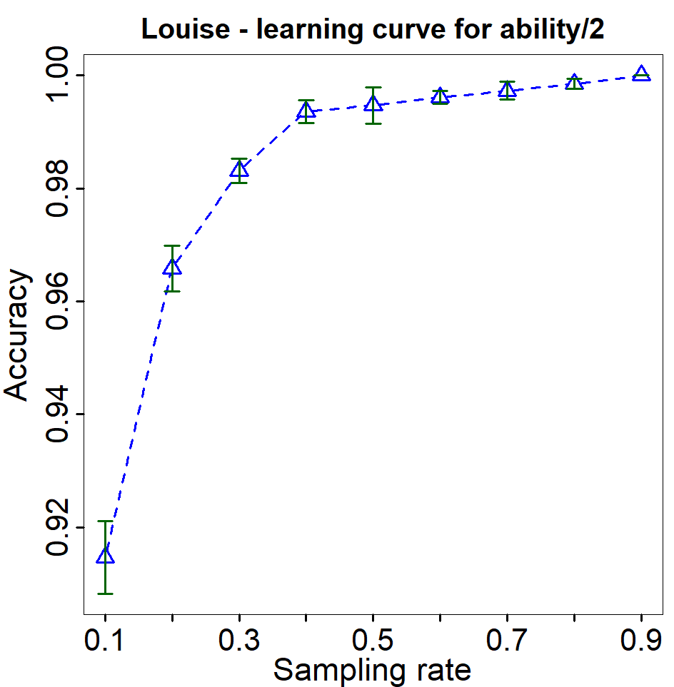

Further documentation

More information about Louise, how it works and how to use it is coming up in the project's manual. For the time being, you can peruse the structured comments in the project's source files. It's also possible to generate a .pdf file from structured documentation, as follows:

Load the project as usual.

Load the doc/latex/maket_tex.pl module:

?- use_module(doc/latex/make_tex).
true.

Run the following query to generate latex files from structure documentation in the project's source code:
```
?- make_tex.
true.
```
Pass the main latex documentation file to pdflatex. By default the main documentation file is louise/doc/latex/documentation.tex
```
cd /doc/latex/
pdflatex -synctex=1 -interaction=nonstopmode .\documentation.tex
pdflatex -synctex=1 -interaction=nonstopmode .\documentation.tex
```
Run the pdflatex command twice to generate a ToC and bookmarks. You will probably see lots of errors but you will still get a .pdf file. Probably (this hasn't been tested extensively).

Note that the structured documentation included in the Prolog source is a work in progress. Most of the time it is mostly accurate, but there are parts of it that are obsolete. Still- better than nothing.

Additionally to all this you may get some useful information from the current draft of the manual stored in the file MAN.md in the directory louise/doc. Keep in mind that MAN.md is a draft and as such may contain incomplete or inaccurate information. On the other hand, it will probably give a general idea of how to use Louise and what it can do.

Citing Louise

If you decide to use Louise in your own work, you will probably want to cite earlier work that gives more details about it. In that case, you are welcome to use the reference to the original Top Program Construction paper, listed below (in bib format) and which contains the most complete discussion of the Top Program Construction algorithm:

@article{Patsantzis2021,
author = {Patsantzis, Stassa and Muggleton, Stephen},
title = {Top Program Construction and Reduction for Polynomial-Time Meta-Interpretive Learning},
journal = {Machine Learning},
year = {2021},
doi = {https://doi.org/10.1007/s10994-020-05945-w}
}

To clarify, you are not required to cite our work to use Louise. You're also not required to wash your hands after going to the loo, it's just good form to do so :P

Bibliography

S.H. Muggleton, D. Lin, N. Pahlavi, and A. Tamaddoni-Nezhad. Meta-interpretive learning: application to grammatical inference. Machine Learning, 94:25-49, 2014
S.H. Muggleton, D. Lin, and A. Tamaddoni-Nezhad. Meta-interpretive learning of higher-order dyadic datalog: Predicate invention revisited. Machine Learning, 100(1):49-73, 2015
S.H. Muggleton. Inductive Logic Programming. New Generation Computing, 8(4):295-318, 1991
S. Patsantzis and S. H. Muggleton. Top Program Construction and Reduction for Polynomial-Time Meta-interpretive Learning. Machine Learning, 2021
S. Patsantzis and S. H. Muggleton. Meta-Interpretive Learning as Metarule Specialisation. Machine Learning, 2021

Cheap and reliable Node.js hosting starts at $3/month, and $1/month static HTML hosting

stassa / louise

Programming Languages