Machine-learning-roadMap

[Machine Learning is the] field of study that gives computers the ability to learn without being explicitly programmed. —Arthur Samuel, 1959

Repository containing a portfolio of machine learning projects and weekly progress towards becoming better at Machine Learning algorithms.

Week 1

Pick a language, and in my opinion, Python is the best for this.

Why? Easy syntax, extensive documentation, great community, availability of resources.

You can prefer to work on R as well; however, R programming has less popularity compare to python in industry.

Create a GitHub profile and learn Git

Git is a powerful version control system that every single person in the STEM field should learn. GitHub is a way of showing the world you know something. Simply writing, I know Python will not be enough for companies. You have to prove you know the Python by showing your projects.

Week 2

Data Analyse Libraries

Learn Pandas and NumPy, the two most important data analysis libraries that will help you to deal with the data preprocessing step. Sometimes, you will want to alter the data according to your needs, or even the data you have will include unnecessary information. Thus, these two libraries will help you to prepare the data. In week 3, we will choose a data visualization library.

Learn the following Machine Learning related terms

Supervised Learning | Unsupervised Learning | Semi-supervised Learning | Reinforcement Learning
Feature Extraction | Feature Selection
Noise | Outliers | Garbage Data
Batch Learning | Online Learning
Overfitting | Regularization | Underfitting
Training Dataset | Testing Dataset

Go over the basic calculus

One big misconsumption on Machine Learning that discourages people is Calculus. You don't have to be a Calculus expert to start ML. This step is not necessary unless you want to get into details of the algorithm.

Week 3

Go over the Basic Statistics

Mean | Standard Deviation | Variance
Covariance | Correlation | Normal Distribution

Go over the Basic Linear Algebra

You don't need to be a master in linear algebra. Here are the basic skills that everyone interested in ML should know.

Matrix multiplication, Addition, and Subtraction
Linear Transformation Transpose, identiy matrix, inverse

Learn the basics of matplotlib and seaborn, two most popular data visualization library

Artificial Neurons and Perceptron

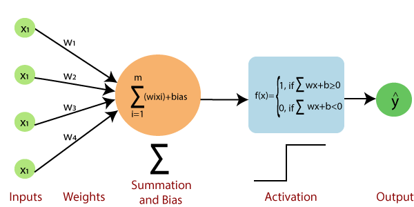
Perceptron is the foundation of neural network. It is supervised algorithm used for binary classifications.

Implementing Perceptron algorithm and fitting Irish dataset to train it

Get yourself familiar with terms: bias, weight, activation function, threshold, convergence.

Common Question

What is the need for bias in the perceptron algorithm?

Weights define how each feature is affective on the classifier, i.e., it only changes the shape of your activation function. However, to be able to shift the activation function along the axis without effecting steepness of it, we need a term bias.

Imagine a situation where both of your features are zero; however, you need an output of 1. No matter which weight you choose, the calculation of the result will be zero. This is where the importance of the bias comes to place. When you have a bias that is always equal to one, you can adjust the weight to get the result of 1.

You can think it as a y-intercept on the line equation: y = mx + b

The weight parameter is 'm' where 'b' stands for the y-intercept of the given x. If you don't have a 'b', your line will always cross the origin which will not be effective in every classifier. To shift the classifier to left or right, we need a y-intercept.

New question is how do we know whether the result of the above calculation will be Yes or Not. In other words, how do we decide which neurons will be fired?

Week 4

Gradient Descent Algorithm

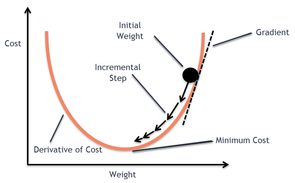
Gradient descent is a famous optimization algorithm that can be used in many areas in machine learning such as clustering, logistic and linear regression. In linear regression, we use GD to find an optimal line that fits the given points in 2D. The main idea is to find the best m(slope) and b(y-intercept) that minimizes the objective function!

Linear Regression

Linear Regression, perhaps one of the fundamental supervised machine learning examples, is an algorithm that uses statistics to predict the corresponding output to the given input based on the previous input-output pairs. The goal is to find the best fit line to the given points. The objective function of the algorithm is the sum of squared errors which we try to minimize.

Week 5

Adaptive Linear Neurons

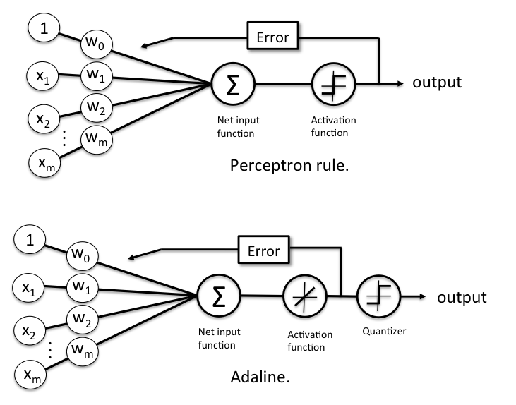
It is an improvement over Perceptron algorithm which uses activation function to update the weights where Perceptron uses unit step function.

In perceptron algorithm, weights are updated after ealuating each sample where ADALINE uses gradient of the whole dataset (objective function) to update the weights.

Stochastic Gradient Descent

It is an optimization technique like Batch Gradient Descent;however, it is more applicable to big dataset. Unlike batch gradient descent, it only picks sample from the given set of features where BGD uses whole dataset.

One-Vs-Rest Strategy

Adaline and Perceptron are binary classifier which can classify 2 classes. Using the one-vs-rest strategy, we can use these binary classifier to a multivariate classifier. For example:

If we have 3 classes (A,B,C), train 3 classifiers. classifierA => class A = 1, classes (B and C) = -1 classifierB => class B = 1, classes (A and C) = -1 classifierC => class C = 1, classes (A and B) = -1

Where classifierA, classifierB, classifierC are the same algorithm (i.e., perceptron)

And to predict the class to which an instance x belongs, it is necessary to predict for each of these n classifiers. classifierA.predict (x) classifierB.predict (x) classifierC.predict (x)

Then, we will take as the class of x where we get the 1.

For example :

classifierA.predict (x) ==> -1 classifierB.predict (x) ==> 1 classifierC.predict (x) ==> -1

The class of x is B.

Week 6

This week, we will get back to Linear Regression, especially to the Multivariate Regression where we have more than one feature.

Label Encoder

Unfortunately, not all the features will have a continuous value all the time. In the case of a categorical feature, we need to convert this into the numbers to be able to use it in our model. Imagine a case where one feature vector contains the following countries: 'Turkey' and 'USA'. You will not able to able to feed this feature to the model. Using the label encoder, we will represent these countries as 0 or 1. For the sake of example, we can represent Turkey as 0 and the USA as 1.

One-Hot Encoder

Giving this 0 and 1 representation can mislead the model. It might give the sense of the representation has some sort of order/strength. To prevent this problem, we use a one-hot encoder, which will separate Turkey and the USA into two columns. This is what one-hot encoding is.

Feature Extraction-Backward Elimination

In real life, what do we do when we have garbage? Well, I throw it away. As in real life, when we have a dataset to feed the Machine Learning algorithm, we need to separate the garbage features/columns from the good one. Because of garbage in garbage out.

In machine learning linguistic, this process is called feature extraction. Using the FE, we can extract the data that will have no impact/bad impact on the output of the model. One of the simple ways to do this is Backward Elimination, which uses the hypothesis testing, specifically p-value, to determine what is garbage data.

But why do we need Feature Extraction? Here are a couple of reasons. Decrease the complexity, improved accuracy and performance, and faster training time.

Classification Algorithms

Logistic Regression

Logistic Regression is a classification algorithm that produces a limited range continuous variable using the probability theory(0-1).

K-Nearest Neighbor

Knn, perhaps one of the most straightforward Machine Learning algorithm, is a classification algorithm works in the following steps:

1. Choose the number of neighbors,
2. Get a data point you want to classify,
3. Measure the distance between the data point and the neighbors from the closes neighbors
4. Among these K neighbors, count the number of data points in each category
5. Assign new instance to the majority category

Norms and Distance Metrics

The distance metric is used in both supervised and unsupervised machine learning algorithms to measure the distance between the data point. Using this distance metric, we can assign new data instances to the corresponding categories. Before getting details of it, we need to understand the norm.

In linear algebra, the norm is a function that takes a vector as an input and produces a scalar value that shows how big the vector is. In other words, it is a distance between the vector and origin. Using norms, we can define distance metrics. The most commonly used norms are L1 and L2.

Week 7

Support Vector Machines

The goal of the SVM is to find the best line that classifies the data points.

SVM has three cases.

The first case is when two classes can be separable with an optimal hyperplane. Pretty boring

The second case is when we relax our model and accept some misclassified instances. This is also known as smooth SVM

The third case is when there is absolutely no way to find an optimal hyper line. In this case, we use kernel tricks to expand the two-dimension into third (Z). When we transform data points to the third dimension, we can find a line to separate them. (Mad respect). Actually, with Radial kernel, even transformation into an infinite dimension possible, but let's not talk about it.

Week 8

Decision Tree

Decision Tree is a supervised learning algorithm that can utilize both prediction and classification. The main goal of the algorithm is to divide until you reach pure data points.

In the form of a tree structure where each node is either: (1) a leaf node, indicating a class of instance or
(2) a decision node, specifying a test to be carried out on a single attribute value, with one branch and a sub-tree for each possible outcome of the test

Overfitting

In machine learning algorithms, we usually fit the training dataset to the created model. Overfitting occurs when the model works well with the training dataset; however, it produces poor performance on the new instances, a.k.a. test dataset. The signal is the underlying pattern that we want our classifier to learn, whereas noise is irrelevant data points. When your classifier learns the noise rather than a signal, it can't do well on the test dataset.

The decision tree algorithm very likely to get affected by overfitting issues. There are a couple of techniques to overcome this issue. The size of the tree has great impact on the accuracy of the model. One of the optimization technique used in DT is to find the optimal max_leaf_nodes which will help our us to get better accuracy. Here is a useful python script.

def get_accuracy(max_leaf_nodes, train_X, val_X, train_y, val_y):
    model = DecisionTreeClassification(max_leaf_nodes=max_leaf_nodes, random_state=0)
    model.fit(train_X, train_y)
    preds_val = model.predict(val_X)
    acc = accuracy_score(val_y, preds_val)

Pruning

Bias and Variance

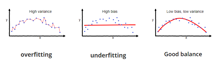
Bias is the difference between the predicted and actual data points. High bias leads to an underfitting issue, which indicates the simplicity of the model.

Variance is the variability of model prediction for a given dataset. High variance leads to overfitting issue, which indicated the classifier concentrated more on the training dataset.

In Machine Learning algorithms, our purpose is to find a sweet spot between them and minimize both bias and variance as low as we can.

Random Forest

Decision tree is simple and easy to interpret;howerver, once it comes to practice, they are not as good as we want them to be. Morelikely, you will encounter overfitting issue.

Random forest is a supervised ML algorithm that utilizes the ensemble learning method. It creates many decision tree at training and uses majority vote technique to classify the new sample!

Algorithm Steps

1. Build a random bootsrap by drawing sample size of n.    
2. At each node   
    2.a Randomly select d features without replacement.    
    2.b Split the node using the features(selected)    
3. Repeat 1-3 k times    
      4. Use majority of vote to assign a class label    

Week 9

Cross Validation

When we work on the Machine Learning algorithm, we split the dataset (namely X), into training and test samples. Using some portion of the dataset to train and again some portion of the SAME dataset to test the dataset. When we use this approach, the maximum portion we will get to test the model is 20% or 30% which is not the optimal number. We want our model to be solid to the unseen dataset.

Using the cross-validation techniques, we can find the optimal accuracy we can receive using the particular dataset on a particular model. Say you have two classification models and you want to know which one will give the optimal result. Using cross-validation, you can figure out which algorithm gives a better result.

Some CV techniques are K-cross validation, leave-one-out CV and stratified K-fold CV.

Pipeline

The purpose of the pipeline is to assemble several steps that can be cross-validated together while setting different parameters. It reduced code size easily by 60% and while increasing the efficiency! Imagine a sitution where you have both numerical and categorical variables (includes NaN values). You need to impute both missing values and apply one hot encoder / dummy variables on the categorical data before feeding your dataset to the algorithm. Doing all of the above steps seperately will make your code ugly and inefficient.

Here the simple steps you can take. Example program can be found at

categorical_cols = [cname for cname in X_train_full.columns if
                    X_train_full[cname].nunique() < 10 and 
                    X_train_full[cname].dtype == "object"]

 # Select numerical columns
 numerical_cols = [cname for cname in X_train_full.columns if 
                X_train_full[cname].dtype in ['int64', 'float64']]

 #Imputer for Numerical Data
 numerical_transformer = SimpleImputer(strategy = 'median')

 #Imputer for Categorical Data
 categorical_transformer = Pipeline(steps = [('imputer', SimpleImputer(strategy = 'most_frequent')),
                                     ('onehot', OneHotEncoder(handle_unknown = 'ignore'))])

 #bundle preprocessing for numerical and categorical data
 preprocessor = ColumnTransformer(transformers=[('num', numerical_transformer, numerical_cols),
                                          ('cat', categorical_transformer, categorical_cols)])
 
 #Create Model
 model = RandomForestRegressor(n_estimators=150, random_state=0)
 
 #Train your model
 clf.fit(X_train, y_train)

 clf = Pipeline(steps=[('preprocessor', preprocessor),
                 ('model', model)])

Classification Evalution Metrics

The most common metric used in classification is accuracy which often leads people to misevaluate their models. In real life, the dataset most likely will not be perfectly distributed, i.e., imbalanced dataset. Imagine a classifier that classifiy either person has fatal desease called Xkiller and classifies 5 out of 800 people infected while others not infected.

When you use this classifier to predict who has the desease or not, your accuracy will be always high altough it will have really small percentrage of correctly identifying the sick person (TP rate). When we have an imbalanced dataset, it is better to use different evaluation metrics.

Recall == Sensitivity == True Positive Rate

What proportion of the actual positives was actually identified correctly?

TP / TP + FN

Precision

What proportion of the positive identification was correct?

TP / TP + FP

Week 10

Data Leakage

The goal of machine learning is to create a model that performs well in terms of accuracy measurement on unseen data. The problem starts with the word "unseen". We don't have the unseen data to train the model and make sure it will give good output. Thus, we perform a train-test split which helps us to test the model on the 'testing' dataset. The purpose here is to see how well the model is generalized on unseen data. Now, the next level is model production. It is when your model will see the real unseen data.

The problem arises when your model performs poorly on the production level. You might be having 95+ accuracy on both tests and training but the accuracy you receive on production level is way below than it. If this is the case, you are a victim of "Data Leakage".

So, data leakage happens when you train your model with a feature that will not be available at the time of prediction. Think a situation where you are building a model that will decide whether a person loan request will be accepted or rejected. One of the feature you have is "Number of Late Payment Notification" which is highly correlated with the prediction. When a person applying the load for the first time, the compony will not have this information and simply will try to guess it which might end up really costly for the compony.

Hyper-paramater Tuning

Grid search is a brute-force exhaustive search paradigm. We specify a list of values for different hyperparameters. The computer evaluates the model performance for each combination of those to obtain the optimal combination of parameter values.

Week 11

Dimensionality Reduction

When the dimension of the dataset is large, the speed of the algorithm as well as the outcome quality will be decreasing. Feature selection and Feature Extraction are two mainly used technique to reduce the number of feature in a dataset.The goal of the feature selection is to drop some of the columns which may result in loosing the helpful feature. On the other hand, feature extraction is a technique which aims to reduce the number of dimension while preserving the insight of the original dataset by projecting the data onto new feature space.

PCA, LDA, KPCA

PCA so far the most widely used dimensionality reduction technique. PCA identifies the axis that contains the largest amount of the variance. To find these components, it uses SVD, a matrix factorization technique. After you find the first d PCA's of the original dataset (usually represented by k), you can reduce the dimension to d by projecting it to hyperlane that defined by first d principal components.

To do this, simply take the dot product of standardized X and V (principal components)

How to choose the right number of dimensions using scikit-learn?

pca = PCA(n_components = 0.95)
X_reduced = pca.fit_transform(X_train)

The parameter n_components means choose the right dimension that preserves the 95% of the original variance in the data!

Another option is to use Elbow method to plot explained_variance_ratio_

Week 12

Regression Analysis

Linear regression is a supervised algorithm that aims to model the relationship between dependent and independent variables by fitting an optimal line. Some regression algorithms are ridge, logistic, decision tree regression and more.

Interview Preperation