Atcold / Pytorch Ppuu
Labels
Projects that are alternatives of or similar to Pytorch Ppuu
Prediction and Policy-learning Under Uncertainty (PPUU)
Gitter chatroom, video summary, slides, poster, website.
Implementing Model-Predictive Policy Learning with Uncertainty Regularization for Driving in Dense Traffic in PyTorch.
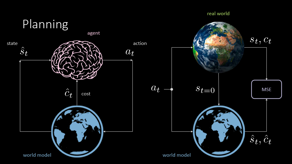
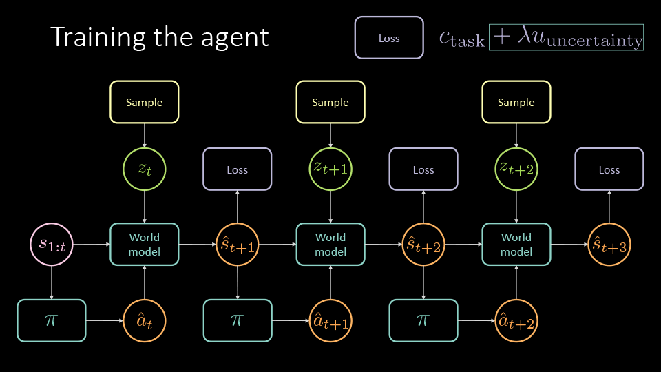
The objective is to train an agent (pink brain drawing) who's going to plan its own trajectory in a densely (stochastic) traffic highway. To do so, it minimises a few costs over trajectories unrolled while interacting with a world model (blue world drawing). We need to start, then, by training the world model with observational data from the real world (Earth's photo), which needs to be downloaded from the Internet.
Getting the real data
To get started, you need to fetch the real world data. Go to this address, and download the TGZ file (330 MB) on your machine. Open a terminal, go to the location where you've downloaded the file, and type:
tar xf xy-trajectories.tgz
This will expand the NGSIM (Next Generation Simulation) data set compressed archive, consisting of all cars trajectories for the 4 available maps (now 1.6 GB). Its content is the following:
xy-trajectories
├── i80
│   ├── trajectories-0400-0415.txt
│   ├── trajectories-0500-0515.txt
│   ├── trajectories-0515-0530.txt
│   └── trajectory-data-dictionary.htm
├── lanker
│   ├── trajectories-0830am-0845am.txt
│   ├── trajectories-0845am-0900am.txt
│   └── trajectory-data-dictionary.htm
├── peach
│   ├── trajectories-0400pm-0415pm.txt
│   ├── trajectories-1245pm-0100pm.txt
│   └── trajectory-data-dictionary.htm
└── us101
    ├── trajectories-0750am-0805am.txt
    ├── trajectories-0805am-0820am.txt
    ├── trajectories-0820am-0835am.txt
    └── trajectory-data-dictionary.htm

4 directories, 14 files
Finally, move the xy-trajectories directory inside a folder named traffic-data.
Setting up the environment
In this section we will fetch the repo, install the dependencies, and view the data we just downloaded, so that we can see if everything runs fine. So, open up your terminal, and type:
git clone [email protected]:Atcold/pytorch-PPUU.git
# or with the https protocol
# git clone https://github.com/Atcold/pytorch-PPUU
Now move (or symlink) the traffic-data folder inside the repo:
cd pytorch-PPUU
mv <traffic-data_folder_path> .
# or
# ln -s <traffic-data_folder_path>
Now install the PPUU environment (this expects you have conda on your system, go here if this is not the case):
conda env create -f environment.yaml
#
# To activate this environment, use:
# > source activate PPUU
#
# To deactivate an active environment, use:
# > source deactivate
#
As prescribed, activate it by typing:
source activate PPUU  # or
conda activate PPUU
Finally, have a look at the four maps available in the NGSIM data set, namely: I-80, US-101, Lankershim, and Peachtree. There is a "bonus" map, called AI, where I've hard coded a policy for the vehicles, which are using a PID controller. Type the following command:
python play_maps.py -map <map>
# where <map> can be one of {i80,us101,peach,lanker,ai}
# add -h to see the full list of options available
The frame rate should be greater than 20 Hz. Often it will be larger than 60 Hz. To be noted, here the vehicles are performing the actions extracted from the trajectories, and not simply following the original spatial coordinates.
Dumping the "state, action, cost" triple
In order to train both the world and agent models, we need to create the observations, starting from the NGSIM trajectories and the simulator. This can be done with the following command:
for t in 0 1 2; do python generate_trajectories.py -map i80 -time_slot $t; done
# to dump the triple for the i80 map, otherwise replace i80 with the map you want
Upon the script termination, we will find a folder named state-action-cost within our traffic-data.
The content of the latter is now the following:
traffic-data/
├── state-action-cost
│   └── data_i80_v0
│       ├── trajectories-0400-0415
│       │   ├── car1.pkl
│       │   └── ...
│       ├── trajectories-0500-0515
│       │   └── ...
│       └── trajectories-0515-0530
│           └── ...
└── xy-trajectories
    └── ...
Additional info
Each pickled vehicle observation is stored as
car{idx}.pkl. Its content is adictwhich includes the items and corresponding sizes (shapes):images (309, 3, 117, 24) actions (309, 2) lane_cost (309,) pixel_proximity_cost (309,) states (309, 7, 4) frames (309,)For example, this vehicle was alive for 309 frames (time steps). The
imagesrepresent the occupancy grid, which is as large as 4 lanes width (24 pixels, here).
- The R channel represents the lane markings.
- The G channel encodes the position and shape of the neighbouring vehicles.
- The B channel depits our own vehicle.
The
actionsis a collection of 2D vectors, encoding the positive and negative acceleration in both x and y directions. Thelane_costandpixel_proximity_costare the task specific costs (see slides for details). Thestatesencode position and velocity of the current vehicle and the most closest 6 ones: left/current/right lanes, front/back. Finally,framestells us the snapshot time stamp, so that we can go back to the simulator, and inspect strange situations present in the observations.
Finally (this will likely be automated soon, and made avaiable for every map), extract the car sizes for the I-80 map with:
python extract_car_size.py
Training the world model
As we have stated above, we need to start by learning how the real world evolve.
To do so, we train a neural net, which tries to predict what happens next, given that we start in a given state, and a specific action is performed.
More precisely, we are going to train an action conditional variational predictive net, which resembles much a variational autoencoder (VAE) that has three inputs (concatenated sequence of states, images, action) and its output is set to be the next item in the sequence (states, images).
In the code, the world model is shortened as fm, which stands for forward dynamics model.
So, let's train the forward dynamics model (fm) on the observational dataset.
This can be done by running:
python train_fm.py -model_dir <fm_save_path>
Training the cost model
Along with the dynamics model, we have a separate model to predict the costs of state and action pairs, which can be trained by running:
python train_cost.py
Training the agent
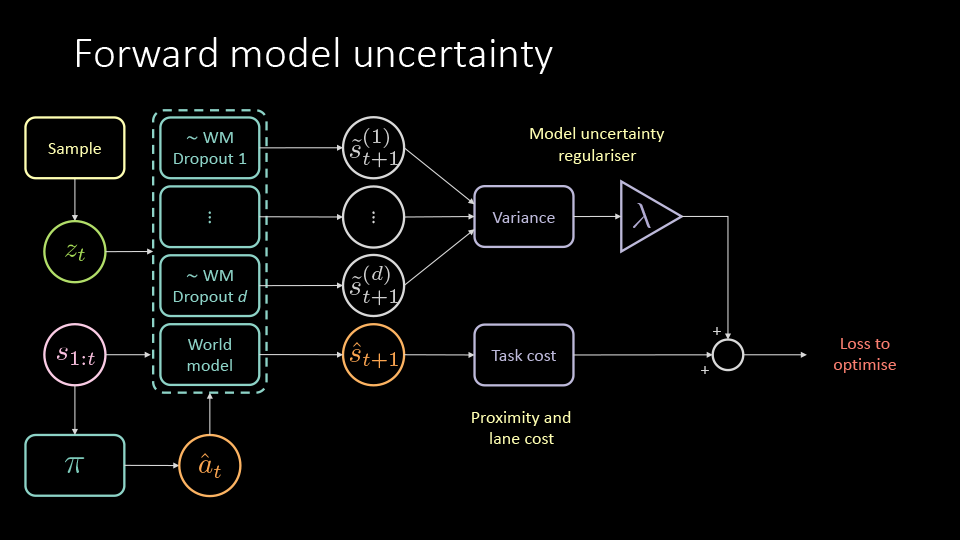
Once the dynamics model is trained, it can be used to train the policy network, using MPUR, MPER, or IL. These corresponds to:
- MPUR: Model-based Policy learning with Uncertainty Regularisation (shown in the figure above)
- MPER: Model-based Policy learning with Expert Regularisation (model-based IL)
- IL: Imitation Learning (copying the expert actions given the past observations)
This is done by running:
python train_{MPUR,MPER,IL}.py -model_dir <fm_load_path> -mfile <fm_filename>
Evaluating the agent
To evaluate a trained policy, run the script eval_policy.py in one of the three following modes.
Type -h to see other options and details.
python eval_policy.py -model_dir <load_path> -policy_model <policy_filename> -method policy-{MPUR,MPER,IL}
You can also specify -method bprop to perform "brute force" planning, which will be computationally expensive.
Parallel evaluation
Evaluation happens in parallel. By default, evaluator script uses min(10, #cores_available) processes. It doesn't go above 10 because then it hits GPU memory limits.
To change the number of processes, you can pass -num-processes argument to eval_policy.py script. Also, for this to work, you need to request cpu cores using --cpus-per-task=X argument for slurm.
The slurm limits cpu usage to 64 cores per user, and gpus to 18 per user, therefore 3 is a reasonable limit to enable us to use all the gpus without hitting the gpu limit when running multiple evaluations. The CPU limit can be extended, but you need to email the IT helpdesk.
Pre-trained models
Here you can download the predictive model and the policy we've trained on our servers (they are bundled together in the model field of this Python dictionary). The agent achieves 82.0% of success rate.
Here, instead, you can download only the predictive models (one for the state and one for the cost), and try to train the policy by your own.


