Loss Landscapes of Regularized Linear Autoencoders

Daniel Kunin, Jonathan M. Bloom, Aleksandrina Goeva, Cotton Seed

Autoencoders are a deep learning model for representation learning. When trained to minimize the distance between the data and its reconstruction, linear autoencoders (LAEs) learn the subspace spanned by the top principal directions but cannot learn the principal directions themselves. In this paper, we prove that L2-regularized LAEs are symmetric at all critical points and learn the principal directions as the left singular vectors of the decoder. We smoothly parameterize the critical manifold and relate the minima to the MAP estimate of probabilistic PCA. We illustrate these results empirically and consider implications for PCA algorithms, computational neuroscience, and the algebraic topology of learning.

ICML paper / poster, arXiv, Talks, Code, Algorithms, Visualization, Neuroscience, Resources, History.

Thoughts? Contact Daniel and Jon (@jbloom22): [email protected], [email protected]

Talks

We presented a 20m talk and poster on June 13 at ICML 2019. Here are the slides.

We're excited to share a primer and seminar given by all four authors at the Models, Inference and Algorithms Meeting at the Broad Institute of MIT and Harvard on February 27, 2019.

We went deeper into Morse theory and ensemble learning at Google Brain on March 6, 2019. Video below left, slides here.

We discussed our latest computational neuroscience results at the Center for Brains, Minds, and Machines at MIT on April 2, 2019. Video below right, slides here, as well as a 20m post-talk interview with zero ferns.

LAE-PCA Algorithms

Here's a simple gradient descent algorithm for LAE-PCA with untied weights (i.e. there is no constraint on W1 or W2):

XXt = X @ X.T
while np.linalg.norm(W1 - W2.T) > epsilon:
    W1 -= alpha * ((W2.T @ (W2 @ W1 - I)) @ XXt + lamb * W1)
    W2 -= alpha * (((W2 @ W1 - I) @ XXt) @ W1.T + lamb * W2)

principal_directions, s,  _ = np.linalg.svd(W2, full_matrices = False)
eigenvalues = np.sqrt(lamb / (1 - s**2))

This may be accelerated on frameworks like TensorFlow using a host of math, hardware, sampling, and deep learning tricks, leveraging our topological and geometric understanding of the loss landscape. For example, one can alternate between exact convex minimization with respect to W1 fixing W2 and then with respect to W2 fixing W1. Or one can synchronize W1 and W2 to be transposes at initialization. Or one can constrain, or tie, W2 = W1.T a priori (see Appendix A):

XXt = X @ X.T
diff = np.inf
while diff > epsilon:
    update = alpha * (((W2 @ W2.T - I) @ XXt) @ W2 + lamb * W2)
    W2 -= update
    diff = np.linalg.norm(update)

principal_directions, s,  _ = np.linalg.svd(W2, full_matrices = False)
eigenvalues = np.sqrt(lamb / (1 - s**2))

We call this version regularized Oja's rule, since without regularization the update step is identical to that of Oja's Rule. Note that this formulation is not convex.

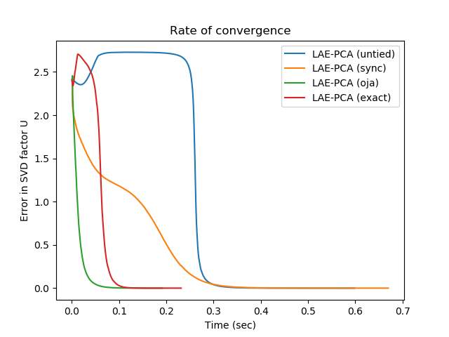
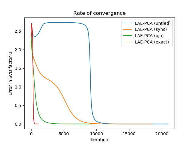
The four variants of the LAE-PCA algorithm described above and runnable examples comparing their convergence rates are here.

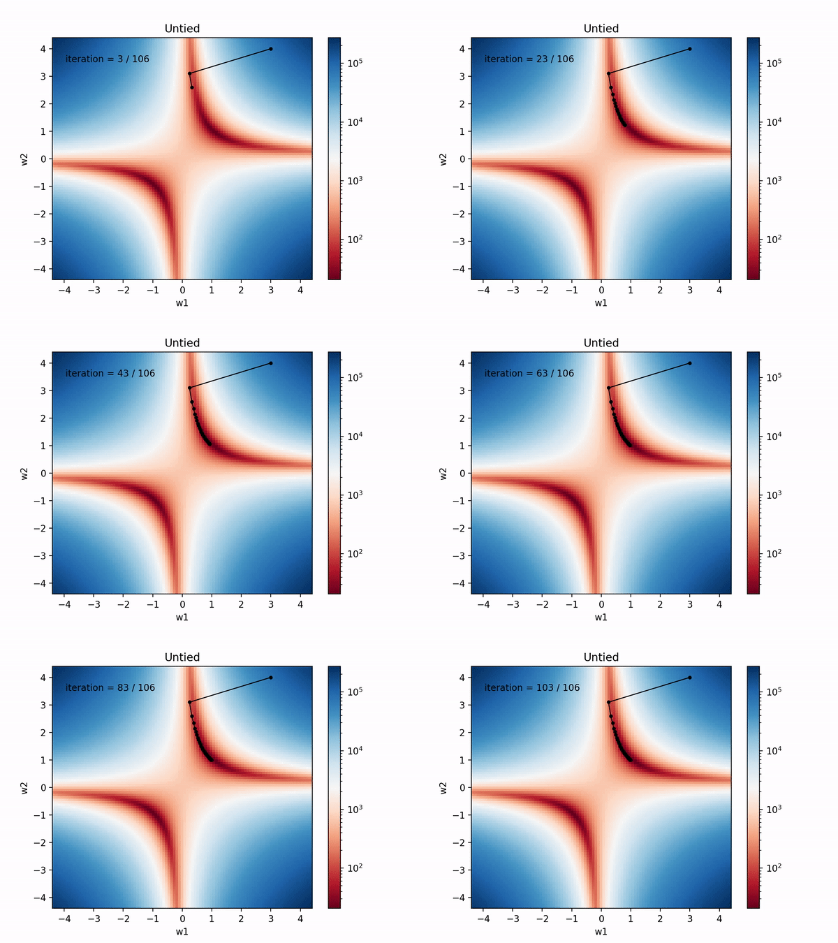
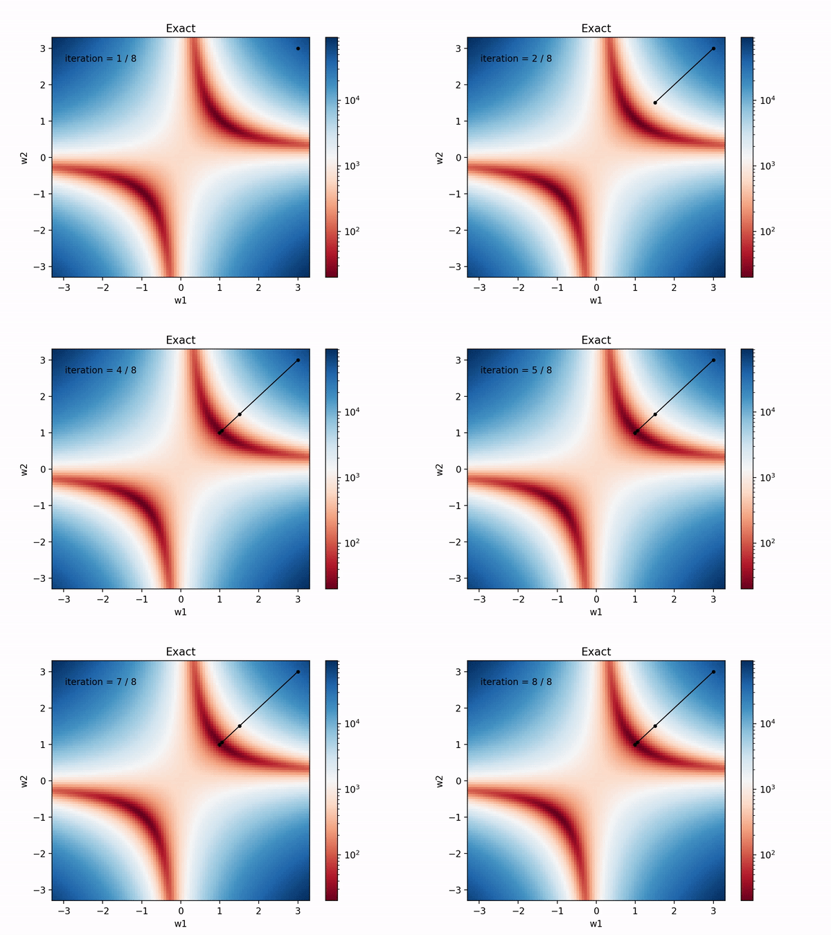
We can visualize the trajectories of these algorithm in the m = k = 1 (scalar) case with code provided here.

Visualization

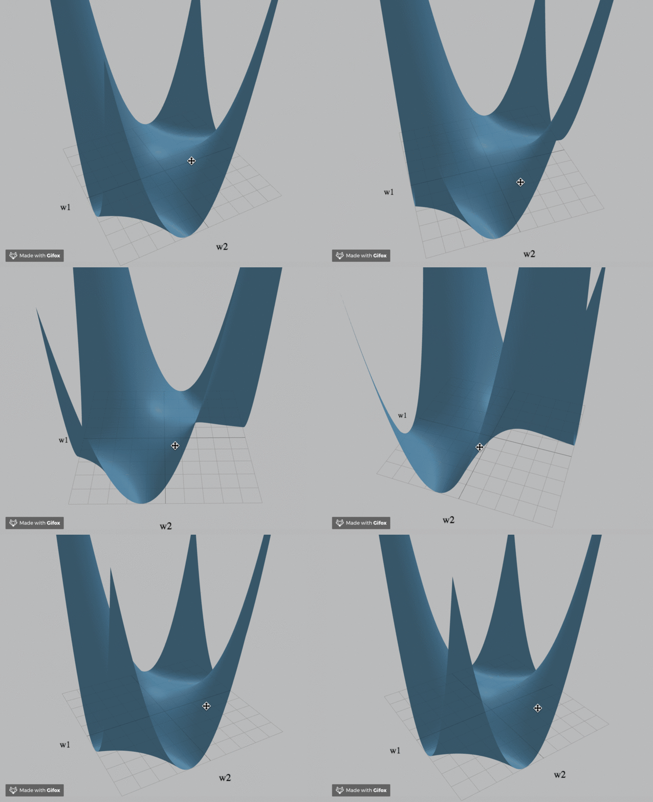
We've created an interactive visualization of the three loss landscapes and more in the m = k = 1 (scalar) case.

Computational Neuroscience

See Jon's talk and interview at the Center for Brains, Minds and Machines for our progress on the computational neuroscience front as of April 2, 2019. Here's the history of how this theoretical project got us thinking about learning in the brain:

In response to v1 of the preprint, Yoshua Bengio wrote us on February 10, 2019 that "the question of obtaining the transpose is actually pretty important for research on a biologically plausible version of backprop, because if you obtain approximate transposes, then several local learning rules give rise to gradient estimator analogues of backprop." He pointed us to his related papers Towards Biologically Plausible Deep Learning and Equivalence of Equilibrium Propagation and Recurrent Backpropagation.

We also found How Important Is Weight Symmetry in Backpropagation? by Poggio, et. al., which calls the "weight symmetry problem [...] arguably the crux of BP’s biological implausibility," as well as the 2018 review Theories of Error Back-Propagation in the Brain which lists weight symmetry as the top outstanding question, going back to Stephen Grossberg, 1987 and Francis Crick, 1989. Discussing the issue with neuroscientist Dan Bear, we believe our work provides a simple, scalable solution to the weight symmetry problem via emergent dynamics.

Dan was kind enough to elaborate on this perspective as follows:

Deep Neural Networks (DNNs) are algorithms that apply a sequence of linear and nonlinear transformations to each input data point, such as an image represented by a matrix of RGB pixel values. DNNs are now widely used in computer vision because they make useful visual information more explicit: for instance, it's hard or impossible to tell what type of object is in an image by training a linear classifier on its pixels or even on the outputs of a shallow neural network; but DNNs can be optimized to perform this sort of "difficult" visual task.

Remarkably, the visual system of our brain seems to use similar algorithms for performing these tasks. Like DNNs, visual cortex consists of a series of "layers" -- in this case, cortical areas -- through which visual information passes. (In fact, the architecture of DNNs was inspired by the neuroanatomy of primate visual cortex.) The action potential firing patterns of neurons in each of these cortical areas can be recorded while an animal is looking at images. Visual neuroscientists have been trying for decades to explain what computations these neurons and cortical areas are doing to allow primates to perform a rich repertoire of behaviors, such as recognizing faces and objects. While they've had some success (for instance in comparing the "early" layers of visual cortex to edge-detection algorithms), neural responses in intermediate and higher visual cortex have been particularly inscrutable -- before 2014, we had no good way of predicting how a neuron in higher visual cortex would respond to a given image.

However, just as the development of DNNs led to a major jump in success at computer vision tasks, these algorithms turned out to be far-and-away the best at explaining neural responses in visual cortex. When shown identical images, the artificial "neurons" in late layers, intermediate, and early layers of DNNs closely resemble the firing patterns of real neurons in late, intermediate, and early visual cortex. (This resemblance is made quantitatively precise by linearly regressing each real neuron on the activation patterns of the DNN "neurons.") This correspondence suggests a general hypothesis about how our visual system processes input: like a DNN, it transforms inputs through a sequence of linear and nonlinear computations, and it has been optimized so that its outputs can be used to perform difficult visual behaviors.

So DNNs and visual cortex seem to share both architecture and function. But this raises another question: do they also share their mechanism of optimization, i.e. a "learning rule?" How do the synapses between neurons in visual cortex become optimized (through a combination of evolution and development) to perform behaviors?

DNNs are typically optimized by stochastic gradient descent on the "weights" of the connections between layers of artificial neurons, which are meant to stand in for synapses between neurons in the brain. Given a set of images and an error function for a particular behavior (such as categorizing objects in each image), the parameters of a DNN are repeatedly updated to minimize the error. Mathematically, this is just the chain rule: calculating how the error depends on the value of each parameter. Since the error is computed based on the output of the network, computing gradients of the error with respect to parameters in the early layers involves "backpropagating" through the intervening layers. Hence the name "Backprop."

Backprop has proven wildly successful at optimizing DNNs. It's therefore an obvious candidate for the learning rule that modifies the strength of synapses in visual cortex. However, running the Backprop learning algorithm requires that artificial neurons in early layers "know" the weights of connections between deeper layers (a specific example: in a two-layer network, the gradient of the error with respect to the first connection weight matrix would depend on the transpose of the second connection weight matrix). This makes neurobiologists worried, because we don't know of a way that some neurons might convey information about the synapse strength of other neurons. (This doesn't mean there isn't a way, we just don't know of one.) Theorists have tried to get around this by proposing that a second set of neurons sends learning signals from higher to lower layers of the brain's visual system. Anatomically, there are plenty of neural connections from later to earlier visual cortex. But we don't know if the signals they send are consistent with what they'd need to if they were implementing Backprop. If they were consistent, it would mean that the transpose of the forward synaptic strengths were somehow encoded in the firing patterns of these backward connections. So how would this set of neurons get access to the synaptic properties of a physically distinct set of neurons?

I think your result offers a potential solution. Imagine that in addition to the usual neurons the compute the "forward pass" of some visual computation, there's an additional set of neurons at each "layer" of the network (i.e. in each area of visual cortex.) These neurons fire in response to inputs from higher layers. So now for every set of connections from layer L to layer L+1, you have a different set of connections from layer L+1 to layer L. In general there need not be any relationship between the forward and the backward weights. But in the special case where they are transposes of each other, this new set of neurons receiving input from layer L+1 will encode the error signal needed to perform Backprop.

It seems like you can now set up a single neural network where this transpose condition is guaranteed to hold. First build your ordinary DNN. Then at each layer, add an equal number of new artificial neurons. These new neurons will receive connections from the original set of neurons at layer L+1. During training, you will minimize both the usual error function (which depends directly only on the output layer) and the reconstruction error, at each layer, between the old neurons and the new neurons. Now the original neurons at layer L+1 are playing the role of the latent state of an autoencoder between the original and the new neurons at layer L. If you apply an L2 regularization to the forward and backward weights then your theorem seems to guarantee that the forward and backward weights will be transposes. Now you no longer need to use the Backpropagation algorithm to update the weights at each layer: at each weight update for layer L, you apply the changes that the Backprop formula tells you to apply, but now it's only a function of the forward and backward inputs to that layer. It's local, and doesn't require neurons to "know about" the synaptic connections in other parts of the network.

L2 regularization also has several possible biological interpretations: in the network I just described, it penalizes synapse strength for being large. Synaptic transmission is energy intensive due to membrane vesicle fusion and production, as well as maintaining transmembrane ion gradients and pumping released neurotransmitter back into the synaptic terminal and vesicles. Stronger synapses require all of these things, so are more energy intensive. Thus, the L2 penalty on synapse strength could be interpreted as an energy cost on the physical building blocks that constitute a functional synapse.

Here is a second interpretation: during training of a neural network, L2 regularization on the weights will cause them to decay exponentially to zero (unless updated due to the other error functions.) In the network I proposed above with L2-regularized linear autoencoders operating between each pair of adjacent layers, the layer-wise reconstruction errors were assumed to be minimized at the same time as the task-related error. But this doesn't need to be the case either in deep learning or in the brain. The reconstruction error could be minimized as part of a faster "inner loop" of optimization, implemented by the local recurrent circuits ubiquitous in cortex or by biophysical mechanisms operating in individual neurons. In this scenario, L2 regularization on the faster timescale could stand in for another well-known neurophysiological phenomenon: the short-term depression of synaptic strength when a neuron fires many action potentials in a short time window, which results from depletion of readily releasable synaptic vesicles and from modifications to synaptic ion channels.

Regularization may therefore play a crucial role in shaping the computations that neural systems perform. A well-known example of this idea in computational neuroscience is the result of Olshausen and Field (Nature 1996). They showed that an autoencoder with an L1 regularization penalty on the activations of the latent state could explain one of the most robust findings in visual neuroscience, the preferential response of primary visual cortical neurons to oriented gratings. The L1 regularization was crucial for producing this effect, which the authors thought of as a "sparse" encoding of natural images. Other forms of biophysical processes have been proposed to explain characteristic features of retinal neuron responses, as well (Ozuysal and Baccus, Neuron 2012.) In biology, the features of any system must be explained as the result of evolutionary constraints. Linking biophysical mechanisms to neural computation is a promising road to understanding the intricacies of the brain.

Reading on DNNs and the primate visual system: https://papers.nips.cc/paper/7775-task-driven-convolutional-recurrent-models-of-the-visual-system.pdf https://www.nature.com/articles/nn.4244

Clear explanation of backpropogation and why it requires the transpose of the forward weight matrix: http://neuralnetworksanddeeplearning.com/chap2.html

Olshausen and Field: https://www.nature.com/articles/381607a0

Useful Resources

Wikipedia has articles on PCA, SVD, autoencoders, regularization, orthogonality, definiteness, matrix calculus, gradient flow, topology, manifolds, Grassmannians, CW complexes, algebraic topology, homology, cellular homology, Morse theory, Morse homology, and random matrix theory.

For a rigorous treatments of manifolds and Morse theory, see Jon's review, Milnor's classic Morse Theory, Banyaga and Hurtubise's Lectures on Morse Homology, and Chen's history of the field through Morse, Thom, Smale, Milnor and Witten. These works are complemented by the development of simplicial, singular, and CW homology in Hatcher's Algebraic Topology. Jon fantasizes that extending Morse homotopy to manifolds with boundary may one day be useful as well...

Project History

Daniel interned with Hail Team at the Broad Institute of MIT and Harvard in Summer 2018. While the four of us were exploring models of deep matrix factorization for single-cell RNA sequencing data, Jon came across v1 of Elad Plaut's From Principal Subspaces to Principal Components with Linear Autoencoders and contacted the author regarding a subtle error. Plaut agreed the main theorem was false as stated, and in correspondence convincingly re-demonstrated the existence of a fascinating empirical phenomenon. We realized quickly from Plaut's code and the scalar case that regularization was the key to symmetry-breaking and rigidity; the form of the general solution was also clear and simple to verify empirically. The bulk of our time was spent banging against chalkboards and whiteboards to establish additional cases and finally a unified proof in full generality.