ritest

Stata package to perform randomization inference on any Stata command.

• Install
• Citation
• Changelog
• Media Coverage
• FAQ

Install

To obtain the latest version through github, from the main window in Stata, run:

net describe ritest, from(https://raw.githubusercontent.com/simonheb/ritest/master/)

If the download from within Stata fails (e.g. because you are behind a firewall),you can always download the files directly:

• https://raw.githubusercontent.com/simonheb/ritest/master/ritest.ado
• https://raw.githubusercontent.com/simonheb/ritest/master/ritest.sthlp

Citation

ritest is not an offical State command. It is a piece of software I wrote and made freely available to the community. Please cite:

Heß, Simon, "Randomization inference with Stata: A guide and software" Stata Journal 17(3) pp. 630-651. [bibtex]

Bugs

There are no known bugs. Please report any unintend or surprising behaviour.

Changelog

• 1.1.8 The savings()-option and the savererandomization()-/saveresampling()-option, now auto-appends the ".dta" and allows to specify ", replace".
• 1.1.4 Added a reject()-option, as permute has it. h/t George s. Ford
• 1.1.2 Fixed the issue that data sanity checks were applied to the full sample, even if and [if] or [in]-statement was used to restrict analysis to a subsample. h/t Fred Finan
• 1.1.0 Added an option (fixlevels()) to constrain re-randomization to certain values of the treatment variable. This can be used for pairwise tests in multi-treatment experiments, by restricting permutation to only some treatment arms.
• 1.0.9 Added the strict and the eps option to the helpfile and added parameter-checks so that "strict" enforces "eps(0)". h/t Katharina Nesselrode
• 1.0.8 Minor bugfix and I got rid of the google analytics part
• 1.0.7 Kason Kerwin pointed out that when string variables were used as strata or cluster ids, all observations were treated as belonging to the same. This is fixed with this version. Also I sped up execution time by dropping unneeded code.
• 1.0.6 Jason Kerwin pointed out an issue with the "saveresampling()"-option. This version fixes this.
• 1.0.4 David McKenzie pointed out that under some conditions, the random seed was ignored. This is fixed with this version.
• 1.0.3 Is the version that was published in the Stata Journal.

Media Coverage

• Finally, a way to do easy randomization inference in Stata! (blog post by David McKenzie)
• Simon Heß has a brand-new Stata package for randomization inference (blog post by Jason Kerwin)

Disclaimer of Warranties and Limitation of Liability

Use at own risk. You agree that use of this software is at your own risk. The author is optimistic but does not make any warranty as to the results that may be obtained from use of this software. The author would be very happy to hear about any issues you might find and will be transparent about changes made in response to user inquiries.

FAQ

1. Exporting Results
2. Call margins or other Pre/Post-Estimation Commands Before ritest, Using Wrappers
3. Using ritest with a Difference-in-Differences Estimator
4. Multiple Treatment Arms
5. Interpreting ritest Output
6. Confidence intervals

How do I export ritest results to TeX/CSV/... with esttab/estout?

run ritest:

eststo regressionresult: reg y treatment controls 
ritest treatment _b[treatment]: `e(cmdline)'

extract the RI p-values:

matrix pvalues=r(p) //save the p-values from ritest
mat colnames pvalues = treatment //name p-values so that esttab knows to which coefficient they belong 
est restore regressionresult        

display the p-values in the table footer:

estadd scalar pvalue_treat = pvalues[1,1]
esttab regressionresult, stats(pvalue_treat)

alternatively, display the p-values next to the coefficient

estadd matrix pvalues = pvalues
esttab regressionresult, cells(b p(par) pvalues(par([ ])))

As a test statistic, I want to use something that requires several steps to be computed, instead of a simple coefficient estimate. E.g. a margins result.

Use a wrapper!

In most cases, randomization inference will be based on observing the same coefficient estimate across different realizations of a treatment assignment. Even in nonlinear models (such as probit), inference on the point estimate often suffices. If not, you can also let ritest call a wrapper function that executes additional commands, like margins:

program margin_post_wrapper
     syntax , command(string)
     `command'
     margins, dydx(_all) post
     //if the command you want to use does not "post" the results, you can make your wrapper programm "eclass" and use "estadd" to post something yourself.
end
ritest treatment (_b[treatment]/_se[treatment]): margin_post_wrapper, command(logit y x treatment)

Of course, you can still beef this up, by passing other arguments to the wrapper to make it more general. Whether or not this makes sense, depends entirely on your context. This may, for example make sense if you are not interested in plain coefficient estimate, but an interaction.

Can you give a simple example using ritest with a difference-in-differences regression?

Setup: binary treatment and panel data.

This won't work:

gen treatpost = treatment*post
ritest treatment _b[treatpost]: reg y treatment post treatpost

for two reasons:

• ritest will keep permuting treatment, but is not aware that treatpost will need to be updated as well.
• ritest does not know that treatment has to be held constant within units.

instead run:

ritest treatment _b[c.treatment#c.post], cluster(unit_id): reg y c.treatment##c.post

I have 3 treatment arms. How do I use ritest?

Setup: There are three treatment arms (0=Control, 1=Treatment A, 2=Treatment B).

What do yo want to test? David McKenzie has a short discussion of this here. In short, there are three main hypotheses one might want to test. (a) Treatment A is no different from Control, (b) Treatment B is no different from Controls and (c) the two treatments are indistinguishable.

Here give an example for (a). (b) and (c) are conducted analogously. First, make sure that you define a single treatment varaible that encodes all three cases as above. Then you can either run:

ritest treatment _b[1.treatment], .... : reg y i.treatment if treatment != 2

or

ritest treatment _b[1.treatment], fixlevels(2)  .... : reg y i.treatment

(for this you'll need the latest version of ritest)

The two variants are slightly different. The first one drops observations of Treatment B from the estimation, assuming they are useless for identifying differences between Treatment A and control. The second one keeps these observations in the estimation sample, but excludes them from the re-randomization. Keeping them in the estimation and re-randomization would make no sense, as this would pool Treatment B and the control group and thus test a weird hypothesis.

The two variants could lead to different results if the observations of group B affect the estimation of _b[1.treatment]. Sometimes this can be good; for example, if your regression includes control variables and their coefficients become more precisely estimated when the full sample is used. In turn, the more precisely estimated control variable coefficient improves the estimate _b[1.treatment], which could be advantageous.

How to I read the output?

I will use this example output to explain all elements:

 0: ritest treatment _b[treatment]/_se[treatment], reps(500) strata(block): areg outcome treatment, r abs(block)
 1:      command:  areg outcome treatment, r abs(block)
 2:        _pm_1:  _b[treatment]/_se[treatment]
 3:  res. var(s):  treatment
 4:   Resampling:  Permuting treatment
 5:Clust. var(s):  __000000
 6:     Clusters:  99
 7:Strata var(s):  block
 8:       Strata:  4
 9:
10:------------------------------------------------------------------------------
11:T            |     T(obs)       c       n   p=c/n   SE(p) [95% Conf. Interval]
12:-------------+----------------------------------------------------------------
13:       _pm_1 |   2.362446      14     500  0.0280  0.0074  .0153906   .0465333
14:------------------------------------------------------------------------------
15:Note: Confidence interval is with respect to p=c/n.
16:Note: c = #{|T| >= |T(obs)|}

1. The full command that is re-estimated at every iteration
2. The statistic that is evaluated after each run of the command
3. The variable that is be permuted/re-sampled
4. A string indicating how the variable is permuted/re-sampled
5. The variable that identifies treatment clusters. If none are given Stata will show the name of a tempvar here (__000000)
6. The number of different clusters.
7. The variable that identifies treatment strata.
8. The number of strata
9. The main table

• T(obs) The realization of the test statistic in the data
• c the count of under how many of the re-sampled assignments, the realization of the test-statistic was more extreme than T(obs)
• n the overall count of re-samplings
• p=c/n the actual RI-based p-value, measuring the fraction of extreme realizations
• SE(p) the standard error of that p-value estimate, based on the "sample" of n re-samplings. This does not say much about whether your hypothesis has to be rejected or not and it is mainly a function of how many permutations you choose.
• 95% Conf. Interval this too is an estimated confidence interval for the p-value, i.e. by choosing the number of re-samplings large enough, this can be made arbitrarily tight.

Finally, the notes indicate which hypotheses is tested. It can be changed by choosing an option to estimate one-sided p-values.

How to get confidence bands?

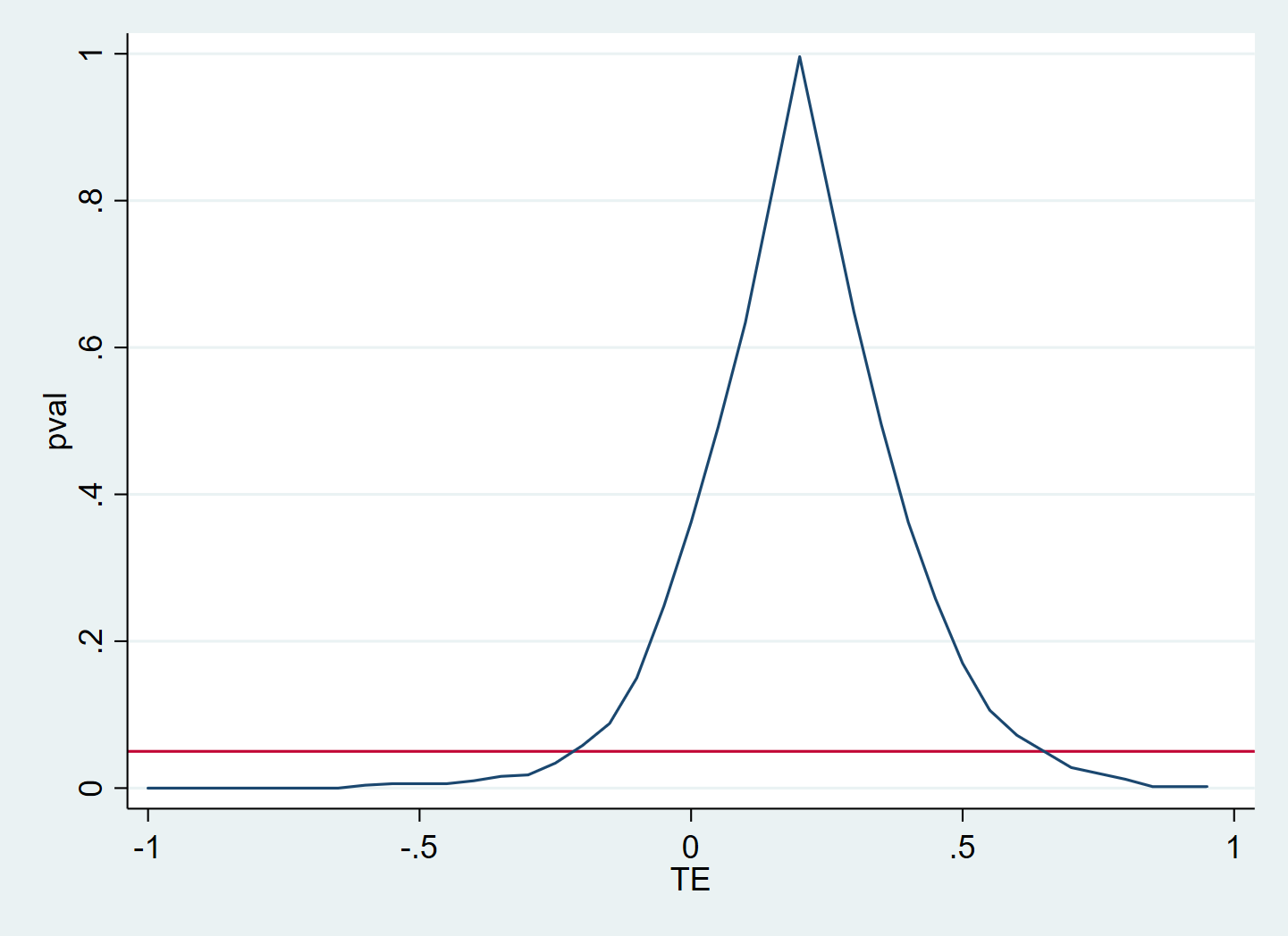
Alwyn Young describes here how to find confidence bands for treatment effect estimates (others discussed this before him, however the paper does a lot more and also gives a nice overiew - I definitely recommend reading it). This involves identifying the set of hypothesized treatment effects that cannot be rejected at a given level. This process can be implemeted by an iterative grid search in Stata. The code below gives a simplistic example of how this could be done with ritest. For a detailed discussion, caveats, and assumptions I recommend consulting Alwyn Young's Paper.

Example code:

//generate mock data
set seed 123
clear
set obs 100
gen treatment = _n>_N/2 //half are treated
gen y = 0.3*treatment + rnormal() //there's a treatment effect
reg y treatment //this is the standard ols result

//run ritest to find which hypotheses for the treatment effect in [-1,1] can[not] be rejected
tempfile gridsearch
postfile pf TE pval using `gridsearch'
forval i=-1(0.05)1 {
	qui ritest treatment (_b[treatment]/_se[treatment]), reps(500) null(y `i') seed(123): reg y treatment //run ritest for the ols reg with the studentized treatment effect
	mat pval = r(p)
	post pf (`i') (pval[1,1])
}
postclose pf

//show results to illustrate confidence intervals
use `gridsearch', clear
tw line pval TE , yline(0.05)

The result will be a dataset of hypothesis tests and corresponding p-values. In this data it is easy to see for which hypothesized treatment effects, the null can be rejected, i.e., the confidence set.

Here I am plotting the p-value against the hypothesized treatment effect. The red line is at 5%, so that the area in which the p-value is higher than the red line corresponds to the 95% confidence set.