antevis / Carnd Project5 Vehicle_detection_and_tracking
Programming Languages
Projects that are alternatives of or similar to Carnd Project5 Vehicle detection and tracking
Vehicle Detection Project
The Goal
To write a software pipeline to identify vehicles in a video from a front-facing camera on a car.
In my implementation, I used a Deep Learning approach to image recognition. Specifically, I leveraged the extraordinary power of Convolutional Neural Networks (CNNs) to recognize images.
However, the task at hand is to not just detect a vehicle presence, but rather to point to its location. Turns out CNNs are suitable for these type of problems as well. There is a lecture in CS231n Course dedicated specifically to localization and the principle I've employed in my solution basically reflects the idea of a region proposal discussed in that lecture and implemented in the architectures such as Faster R-CNN.
The main idea is that since there is a binary classification problem (vehicle/non-vehicle), we can construct the model in such a way that it would have an input size of a small training sample (e.g., 64x64x3) and a single-feature convolutional layer of 1x1 at the top, which output will be used as a probability value for classification.
Having trained this type of a model, the input's width and height dimensions can be expanded arbitrarily, transforming the output layer's dimensions from 1x1 to a map with an aspect ratio approximately matching that of a new large input.
Essentially, this would be equal to:
- Cutting new big input image into squares of the models' initial input size (e.g., 64x64)
- Detecting the subject in each of those squares
- Stitching the resulting 1x1 detections, preserving the same order as the corresponding squares in the source input into a map with the aspect ratio of the sides approximately matching that of a new big input image.
Data
For training I used the datasets provided by Udacity: KITTI-extracted part of vehicles and a corresponding number of samples from non-vehicles, randomly sampled.
The Final model had difficulties in detecting white Lexus in the Project video, so I augmented the dataset with about 200 samples of it. Additionally, I used the same random image augmentation technique as in Project 2 for Traffic Signs Classification, yielding about 1500 images of vehicles from the Project video. The total number of vehicle's images used for training, validation and testing was about 7500.

As mentioned above, equal number of non-vehicles images has been added as a negative examples.
Model
The technique of constructing the top of the network has been borrowed from the implementation of Max Ritter, who apparently employed the same approach.
To derive the final model, I have tested a lot of model architectures with varying complexity.
I started with Transfer Learning from VGG16 with weights trained on ImageNet. VGG is a great and well-tested architecture and ImageNet weights obviously assume that it has an idea of the vehicles features. I added my top single-feature binary classifier and fine-tuned the model. As expected, it yielded a pretty high test accuracy of about 99,5 %. The flip side with the VGG is that it is rather complex, making predictions computationally heavy.
I then tested a number of custom CNN configurations of varying number of layers and shapes and finally arrived at the following model layout:
| Layer (type) | Output Shape | Param # |
|---|---|---|
| lambda_2 (Lambda) | (None, 64, 64, 3) | 0 |
| cv0 (Conv2D) | (None, 64, 64, 16) | 448 |
| dropout_4 (Dropout) | (None, 64, 64, 16) | 0 |
| cv1 (Conv2D) | (None, 64, 64, 32) | 4640 |
| dropout_5 (Dropout) | (None, 64, 64, 32) | 0 |
| cv2 (Conv2D) | (None, 64, 64, 64) | 18496 |
| max_pooling2d_2 (MaxPooling2D) | (None, 8, 8, 64) | 0 |
| dropout_6 (Dropout) | (None, 8, 8, 64) | 0 |
| fcn (Conv2D) | (None, 1, 1, 1) | 4097 |
| Total params: | 27,681 | |
| Trainable params: | 27,681 |
With as little as 27,681 parameters, it still produces the test accuracy of about 99,4%.
607/607 [==============================] - 54s - loss: 0.0764 - acc: 0.8940 - val_loss: 0.0213 - val_acc: 0.9778
Epoch 2/5
607/607 [==============================] - 48s - loss: 0.0194 - acc: 0.9756 - val_loss: 0.0142 - val_acc: 0.9866
Epoch 3/5
607/607 [==============================] - 48s - loss: 0.0117 - acc: 0.9855 - val_loss: 0.0099 - val_acc: 0.9897
Epoch 4/5
607/607 [==============================] - 48s - loss: 0.0075 - acc: 0.9904 - val_loss: 0.0107 - val_acc: 0.9879
Epoch 5/5
607/607 [==============================] - 48s - loss: 0.0063 - acc: 0.9923 - val_loss: 0.0073 - val_acc: 0.9926
Training complete. Weights for best validation accuracy have been saved to ppico_2017_5_13_23_56_41.h5.
Evaluating accuracy on test set.
test accuracy:  [0.0065823850340600764, 0.99373970345963758]
The Model has been implemented in Keras with TensorFlow backend.
The model may be trained directly from the Terminal invoking python model.py. Though training assumes the existence
of the training data in the following folders: samples/vehicles, samples/non-vehicles.
Sample detection results


Transforming the model
The region of interest for vehicle detection starts at an approximately 400th pixel from the top and spans vertically for about 260 pixels. That said, we have a region of interest with the dimensions of 260x1280x3, where 3 is the number of color channels, starting at 400th pixel vertically.
This transforms the Model as follows:
| Layer (type) | Output Shape | Param # |
|---|---|---|
| lambda_2 (Lambda) | (None, 260, 1280, 3) | 0 |
| cv0 (Conv2D) | (None, 260, 1280, 16) | 448 |
| dropout_4 (Dropout) | (None, 260, 1280, 16) | 0 |
| cv1 (Conv2D) | (None, 260, 1280, 32) | 4640 |
| dropout_5 (Dropout) | (None, 260, 1280, 32) | 0 |
| cv2 (Conv2D) | (None, 260, 1280, 64) | 18496 |
| max_pooling2d_2 (MaxPooling2D) | (None, 32, 160, 64) | 0 |
| dropout_6 (Dropout) | (None, 32, 160, 64) | 0 |
| fcn (Conv2D) | (None, 25, 153, 1) | 4097 |
| Total params: | 27,681 | |
| Trainable params: | 27,681 |
As can be seen, the top convolutional layer now has the dimensionality of (? ,25, 153, 1), where 25x53 actually represents a miniature map of predictions that will ultimately be projected to the original hi-res image.
The vehicle detection pipeline has been encapsulated in a dedicated class VehicleScanner in the scanner.py module.
Its instance being initialized within the Detector class (detector.py module). The common Lane + Vehicles
detection process starts with invoking the embedDetections() function of Detector class. This function internally
calls VehicleScanner.relevantBoxes() function to obtain vehicles' bounding boxes (line 201 detector.py).
The undistorted version of the imaged being passed to VehicleScanner.relevantBoxes() as the parameter.


VehicleScanner performs the following tasks:
-
Obtains the region of interest (260x1280 starting with 400th pixel from the top of the image). (line 43 of
scanner.py)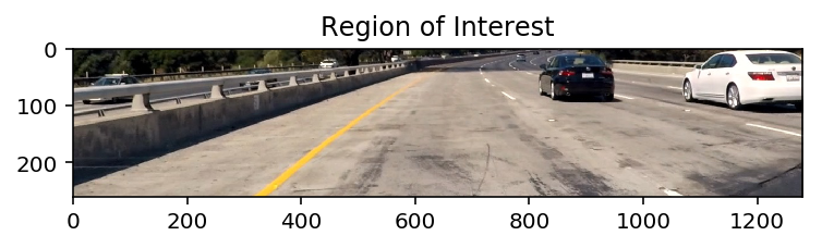
-
Produces the detection map (lines 45 - 52 of
scanner.py):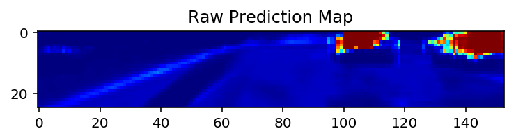 Note the dimensionality is 25x153
 -
Applying the confidence threshold produces the binary map (lines 62 - 65 of
scanner.py):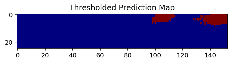 The predictions are actually very polarized, that is, they mostly stick to 1 and 0 for vehicles and
non-vehicle points. That said, the midpoint of 0.5 for a confidence threshold might also to be a
reliable choice.
The predictions are actually very polarized, that is, they mostly stick to 1 and 0 for vehicles and
non-vehicle points. That said, the midpoint of 0.5 for a confidence threshold might also to be a
reliable choice. -
Labels the obtained detection areas with the
label()function of thescipy.ndimage.measurementspackage (line 67 ofscanner.py). This step allows outlining the boundaries of labels that will, in turn, helps to keep each detected island within its feature label's bounds when building the Heat Map. This is also the first approximation of detected vehicles. The output of thelabel()function:


(array([[0, 0, 0, ..., 2, 2, 2],
        [0, 0, 0, ..., 2, 2, 2],
        [0, 0, 0, ..., 2, 2, 2],
        ...,
        [0, 0, 0, ..., 0, 0, 0],
        [0, 0, 0, ..., 0, 0, 0],
        [0, 0, 0, ..., 0, 0, 0]], dtype=int32), 4)
The second item (4) indicates how many features have been labeled in total.
-
These featured labels are being used to project detection points to the coordinate space of the original image, transforming each point into a 64x64 square and keeping those squares within the features' area bounds (lines 69 - 104 of
scanner.py). To illustrate the result of this points-to-squares transformation projected onto the original image: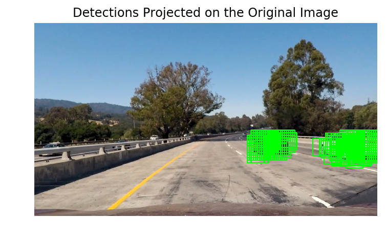
-
Creates the Heat Map. Overlapping squares are essentially building-up the 'heat'. (function
addHeat()ofVehicleScanner, lines 109 - 127 ofscanner.py). Threshold is not applied, as it actually does more harm than good, forcing excessive separation of feature labels with unwanted consequences at the phase of grouping rectangles (see 9.). The model detection accuracy is good enough to be sure that most false positives had been rejected earlier by confidence threshold.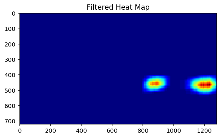
-
The Heat Map is being labeled again, producing the final 'islands' for actual vehicles' bounding boxes (line 141 of
scanner.py):


(array([[0, 0, 0, ..., 0, 0, 0],
        [0, 0, 0, ..., 0, 0, 0],
        [0, 0, 0, ..., 0, 0, 0],
        ...,
        [0, 0, 0, ..., 0, 0, 0],
        [0, 0, 0, ..., 0, 0, 0],
        [0, 0, 0, ..., 0, 0, 0]], dtype=int32), 2)
Although no features are visible in the truncated output, second item indicates that there are 2 islands have been found.
-
Labeled features of the Heat Map are being saved to the
VehicleScanner'svehicleBoxesHistoryvariable, where they would be kept for a certain number of consequent frames (line 176 ofscanner.py). -
The final step is getting the actual bounding boxes for the vehicles.
OpenCVprovides a handy functioncv2.groupRectangles(). As said in docs: "It clusters all the input rectangles using the rectangle equivalence criteria that combines rectangles with similar sizes and similar locations." Exactly what is needed. The function has asgroupThresholdparameter responsible for "Minimum possible number of rectangles minus 1". That is, it won't produce any result until the history accumulates bounding boxes from at least that number of frames (lines 178 - 179 ofscanner.py).

Video Implementation
I've merged Vehicle and Lane detections into a single pipeline to produce a combined footage with both the Lane and
vehicles bounding boxes. It may be invoked directly from the Terminal with python Detector.py.
Here's the result
Discussion
I thoroughly studied the approach of applying SVM classifier to HOG features covered it the Project lessons, but actually intended to employ the Deep Learning approach even before that. In a CS231n lecture that I referred to at the beginning, the HOGs are actually viewed only from a historical perspective. Furthermore, there is a paper which argues that the DPMs (those are based on HOGs) might be viewed as a certain type of Convolutional Neural Networks.
It took some time figuring out how to derive a model that would produce the detection map of a reliable resolution when expanding it to accept the input image of a fully-sized region of interest.
Even the tiny model that I've finally picked takes about 0.75 seconds to produce a detection map for 260x1280x3 input image on a Mid-2014 3GHz quad-core i7 MacBook Pro. That is 1.33 frames per second.