dvgodoy / Deepreplay
Projects that are alternatives of or similar to Deepreplay
Deep Replay
Generate visualizations as in my "Hyper-parameters in Action!" series of posts!
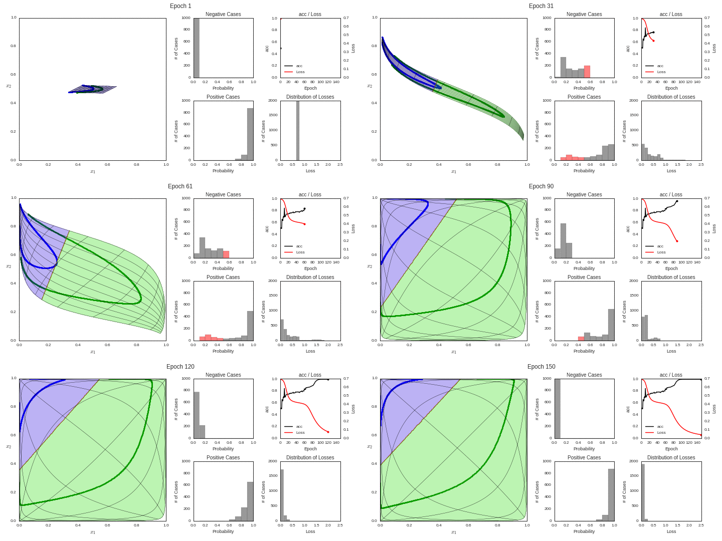
Deep Replay is a package designed to allow you to replay in a visual fashion the training process of a Deep Learning model in Keras, as I have done in my Hyper-parameter in Action! post on Towards Data Science.
This is an example of what you can do using Deep Replay:
It contains:
- a Keras' callback - ReplayData - which collects then necessary information, mostly the weights, during the training epochs;
- a class Replay, which leverages the collected data to build several kinds of visualizations.
The available visualizations are:
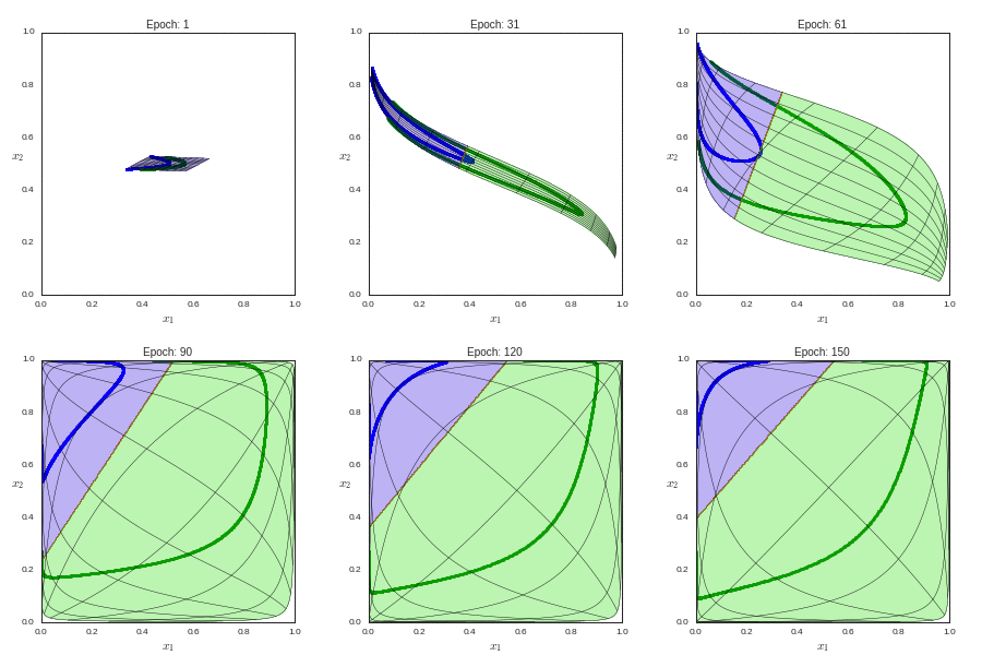
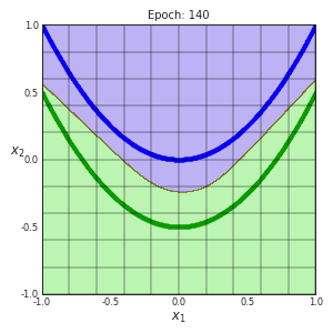
- Feature Space: plot representing the twisted and turned feature space, corresponding to the output of a hidden layer (only 2-unit hidden layers supported for now), including grid lines if the input is 2-dimensional;
- Decision Boundary: plot of a 2-D grid representing the original feature space, together with the decision boundary (only 2-dimensional inputs supported for now);
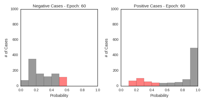
- Probabilities: two histograms of the resulting classification probabilities for the inputs, corresponding to the output of the final layer (only binary classification supported for now);
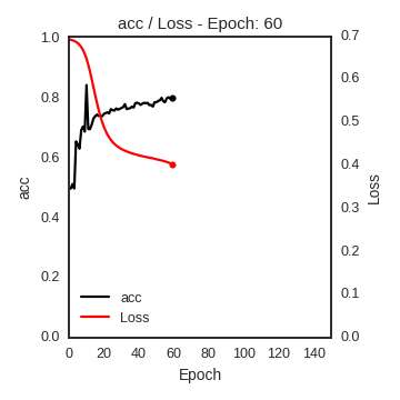
- Loss and Metric: line plot for the loss and a chosen metric, computed over all the inputs;
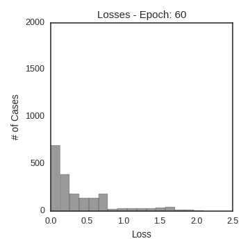
- Losses: histogram of the losses computed over all the inputs (only binary cross-entropy loss suported for now).
| Feature Space | Decision Boundary | Class Probability | Loss/Metric | Losses |
|---|---|---|---|---|
 |
 |
 |
 |
 |
Google Colab
Eager to try it out right away? Don't wait any longer!
Open the notebooks directly on Google Colab and try it yourself:
Installation
To install Deep Replay from PyPI, just type:
pip install deepreplay
Documentation
You can find the full documentations at Read the Docs.
Quick Start
To use Deep Replay, you must first create an instance of the Keras' callback, ReplayData, passing as arguments the inputs (X) and outputs (y) you're using to train the model, as well as the filename and group (for more details, see h5py) where you want the collected data to be saved:
from deepreplay.callbacks import ReplayData
from deepreplay.datasets.parabola import load_data

X, y = load_data()

replaydata = ReplayData(X, y, filename='hyperparms_in_action.h5', group_name='part1')
Then, create a Keras model of your choice, compile it and fit it, adding the instance of the callback object you just created:
from keras.models import Sequential
from keras.layers import Dense
from keras.optimizers import SGD
from keras.initializers import glorot_normal, normal

model = Sequential()
model.add(Dense(input_dim=2,
                units=2,
                activation='sigmoid',
                kernel_initializer=glorot_normal(seed=42),
                name='hidden'))
model.add(Dense(units=1,
                activation='sigmoid',
                kernel_initializer=normal(seed=42),
                name='output'))

model.compile(loss='binary_crossentropy', optimizer=SGD(lr=0.05), metrics=['acc'])

model.fit(X, y, epochs=150, batch_size=16, callbacks=[replaydata])
After your model finishes training, you'll end up with a HDF5 file (hyperparms_in_action.h5, in the example), containing a new group (part1, in the example) that holds all the necessary information. The Keras model itself is also automatically saved as <group_name>_model.h5, that is, part1_model.h5 in the example.
Next, it is time to feed the information to a Replay instance:
from deepreplay.replay import Replay

replay = Replay(replay_filename='hyperparms_in_action.h5', group_name='part1')
Then, you can create a regular Matplotlib figure, like:
import matplotlib.pyplot as plt

fig, ax = plt.subplots(1, 1, figsize=(5, 5))
And use your Replay instance to build the visualization of your choice, say, Feature Space based on the output of the layer named hidden:
fs = replay.build_feature_space(ax, layer_name='hidden')
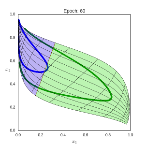
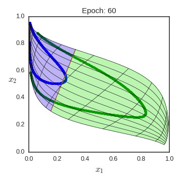
Now, you're ready to make a plot of your Feature Space in any given epoch, or to animate its evolution during the whole training:
fs.plot(epoch=60).savefig('feature_space_epoch60.png', dpi=120)
fs.animate().save('feature_space_animation.mp4', dpi=120, fps=5)
The results should look like this:
TIP: If you get an error message regarding the MovieWriter, try conda install -c conda-forge ffmpeg to install FFMPEG, the writer used to generate the animations.
Alternatively, you can explicitly specify a different MovieWriter, for instance, avconv:
from matplotlib import animation

Writer = animation.writers['avconv']
metadata = dict(title='Sigmoid Activation Function',
                artist='Hyper-parameters in Action!')
writer = Writer(fps=5, metadata=metadata)

fs.animate().save('feature_space_animation.mp4', dpi=120, writer=writer)
FAQ
1. Grid lines are missing!
Does your input have more than 2 dimensions? If so, this is expected, as grid lines are only plot for 2-dimensional inputs.
If your input is 2-dimensional and grid lines are missing nonetheless, please open an issue.
2. My hidden layer has more than 2 units! How can I plot it anyway?
Apart from toy datasets, it is likely the (last) hidden layer has more than 2 units. But DeepReplay only supports FeatureSpace plots based on 2-unit hidden layers. So, what can you do?
There are two different ways of handling this: if your inputs are 2-dimensional, you can plot them directly, together with the decision boundary. Otherwise, you can (train and) plot 2-dimensional latent space.
2.1 Using Raw Inputs
Instead of using FeatureSpace, you can use DecisionBoundary and plot the inputs in their original feature space, with the decision boundary as of any given epoch.
In this case, there is no need to specify any layer, as it will use the raw inputs.
## Input layer has 2 units
## Hidden layer has 10 units
model = Sequential()
model.add(Dense(input_dim=2, units=10, kernel_initializer='he', activation='tanh'))

## Typical output layer for binary classification
model.add(Dense(units=1, kernel_initializer='normal', activation='sigmoid', name='output'))

...

fs = replay.build_decision_boundary(ax_fs)
For an example, check the Circles Dataset.
2.2 Using a Latent Space
You can add an extra hidden layer with 2 units and a LINEAR activation function and tell DeepReplay to use this layer for plotting the FeatureSpace!
## Input layer has 57 units
## Hidden layer has 10 units
model = Sequential()
model.add(Dense(input_dim=57, units=10, kernel_initializer='he', activation='tanh'))

## Added layer with 2 units and LINEAR activation - the layer to plot using FeatureSpace!
model.add(Dense(units=2, kernel_initializer='normal', activation='linear', name='hidden'))

## Typical output layer for binary classification
model.add(Dense(units=1, kernel_initializer='normal', activation='sigmoid', name='output'))

...

fs = replay.build_feature_space(ax_fs, layer_name='hidden')
By doing so, you will be including a transformation from a highly dimensional space to a 2-dimensional space, which is also going to be learned by the network.
In fact, the model will be learning a 2-dimensional latent space, which will then feed the last layer. You can think of this as a logistic regression with 2 inputs, in this case, the latent factors.
For examples, check either the Moons Dataset or UCI Spambase Dataset notebooks.
Comments, questions, suggestions, bugs
DISCLAIMER: this is a project under development, so it is likely you'll run into bugs/problems.
So, if you find any bugs/problems, please open an issue or submit a pull request.

