gdroguski / Gaussianprocesses
Programming Languages
Projects that are alternatives of or similar to Gaussianprocesses
Gaussian Process Regression and Forecasting Stock Trends
The aim of this project was to learn the mathematical concepts of Gaussian Processes and implement them later on in real-world problems - in adjusted closing price trend prediction consisted of three selected stock entities.
It is obvious that the method developped during this process of creation is not ideal, if it were so I wouldn't share this publictly and made profits myself instead. ;) But nevertheless it can give some good forecasts and be used as another indicator in technical analysis of stock prices as we will see later on below.
The project is written in Python 3 and to run it you will need also matplotlib, numpy, pandas and sklearn libraries. As written in Data and Evaluation section, the data was downloaded from yahoo finance section in the csv format so basically if you'd like to test this model on some other companies from yahoo you only have to download and put it into Data directory within the project.
Worth mentioning is the fact that to run the analysis you have to run the data_presenter.py file and the project will do it's magic for every file in Data directory. So to run just type python data_presenter.py.
Table of Contents
-
Gaussian Processes
- Basic Concepts
- Covariance Function
- Hyperparameters Optimization
- Forecasting Methodology
-
Data and Evaluation
- S&P 500 (GSPC)
- The Boeing Company (BA)
- Starbucks (SBUX)
- Summary
- Bibliography
Gaussian Processes
Gaussian processes are a general and flexible class of models for nonlinear regression and classification. They have received attention in the machine learning community over last years, having originally been introduced in geostatistics. They differ from neural networks in that they engage in a full Bayesian treatment, supplying a complete posterior distribution of forecasts. For regression, they are also computationally relatively simple to implement, the basic model requiring only solving a system of linear equations with computational complexity  .
.
This section will briefly review Gaussian processes at a level sufficient for understanding the forecasting methodology developed in this project.
Basic Concepts
A Gaussian process is a generalization of the Gaussian distribution - it represents a probability distribution over functions which is entirely specified by a mean and covariance functions. Mathematical definition would be then as follows:
Definition: A Gaussian process is a collection of random variables, any finite number of which have a joint Gaussian distribution.
Let  be some process
  . We write:

where  and
and  are the mean and covariance functions, respectively:

We will assume that we have a training set  where
where  and
and  . For sake of simplicity let
  be the matrix of all inputs, and
  the vector of targets. Also we should assume that the observations
  from the proces are noisy:

Regression with a GP is achieved by means of Bayesian inference in order to obtain a posterior distribution over functions given a suitable prior and training data. Then, given new test inputs, we can use the posterior to arrive at a predictive distribution conditional on the test inputs and the training data.
It is often convienient to assume that the GP prior distribution has mean of zero

Let  be a vector of function values in the training set
  . Their prior distribution is then:

where  is a covariance matrix evaluated using covariance function between given points (also known as kernel or Gram matrix). Considering the joint prior distribution between training and the test points, with locations given by matrix
  and whose function values are
  we can obtain that

Then, using Bayes' theorem the join posterior given training data is

where  since the likelihood is conditionally independent of given
  , and
, and

where  is
is  identity matrix. So the desired predictive distribution is

Since these distributions are normal, the result of the marginal is also normal we have

where are test points and

The computation of  is the most computationally expensive in GP regression, requiring as mentioned earlier
  time and also
  space.
Covariance Function
A proper choice for the covariance function is important for encoding knowledge about our problem - several examples are given in Rasmussen and Williams (2006). In order to get valid covariance matrices, the covariance function should be symmetric and positive semi-definite, which implies that the all its eigenvalues are positive,

for all functions defined on appropriate space and measure  .
.
The two most common choices for covariance functions are the squared exponential (also known as the Gaussian or radial basis function kernel):

which we will use in our problem and the rational quadratic:

In both cases, the hyperparameter  governs the characteristic length scale of covariance function, indicating the degree of smoothness of underlying random functions and we can interpret as scaling hyperparameter. The rational quadratic can be interpreted as an infinite mixture of squared exponentials with different length-scales - it converges to a squared exponential with characteristic length-scale as
  . In this project has been used classical Gasussian kernel.
Hyperparameters Optimization
For many machine learning algorithms, this problem has often been approached by minimizing a validation error through cross-validation, but in this case we will apply alternative approach, quite efficient for GP - maximizing the marginal likelihood of the observerd data with respect to the hyperparameters. This function can be computed by introducing latent function values that will be integrated over. Let  be the set of hyperparameters that have to be optimized, and
  be the covariance matrix computed by given covariance function whose hyperparameters are ,

The marginal likelihood then can be wrriten as

where the distribution of observations  is conditionally independent of the hyperparameters given the latent function . Under the Gaussian process prior, we have that
  , or in terms of log-likelihood

Since the distributions are normal, the marginalization can be done analytically to yield

This expression can be maximized numerically, for instance by a conjugate gradient or like in our case - the default python's sklearn optimizer fmin_l_bfgs_b to yield the selected hyperparameters:

The gradient of the marginal log-likelihood with respect to the hyperparameters-necessary for numerical optimization algorithms—can be expressed as

See Rasmussen and Williams (2006) for details on the derivation of this equation.
Forecasting Methodology
The main idea of this approach is to avoid representing the whole history as one time series. Each time series is treated as an independent input variable in the regression model. Consider a set of  real time series each of length
  ,
,  ,
,  and
and  . In this application each
  represents a different year, and the series is the sequence of a particular prices during the period where it is traded. Considering the length of the stock market year, usually
  will be equal to
  and sometimes less if incomplete series is considered (for example this year) assuming that the series follow an annual cycle. Thus knowledge from past series can be transferred to a new one to be forecast. Each trade year of data is treated as a separate time series and the corresponding year is used as a independent variable in regression model.
The forecasting problem is that given observations from the complete series  and (optionally) from a partial last series
  ,
,  , we want to extrapolate the last series until predetermined endpoint (usually a multiple of a quarter length during a year) - characterize the joint distribution of
  ,
,  for some
  . We are also given a set of non-stochastic explanatory variables specific to each series,
  , where
  . Our objective is to find an effective representation of
  , with
  and
and  ranging, respectively over the forecatsing horizon, the available series and the observations within a series.
Everything mentioned in this section was implemented in Python using the wonderful library sklearn, mainly the sklearn.gaussian_process.
Data and Evaluation
For this project, three stocks/indices were selected:
- S&P 500 (GSPC),
- The Boeing Company (BA),
- Starbucks (SBUX).
The daily changes of adjusted closing prices of these stocks were examined and the historical data was downloaded in the form of csv file from the yahoo finance section. There are two sample periods taken for these three indices: first based on years 2008-2016 for prediction of whole year 2017 and second based on years 2008-2018 (up to end of second quarter) for prediction of the rest of the 2018 year. We have about 252 days of trading year per years since no data is observed on weekends. However, some years have more than 252 days of trading and some less so we choose to ignore 252+ days and for those with less trading days the remaing few we fill up with mean of the year to have equal  for all years.
We choose to use adjusted close prices because we aim to predict the trend of the stocks not the prices. The adjusted close price is used to avoid the effect of dividends and splits because when stock has a split, its price drops by half. The adjusted close prices are standardized to zero mean and unit standard deviation. We also normalize the prices in each year to avoid the variation from previous years by subtracting the first day to start from zero.
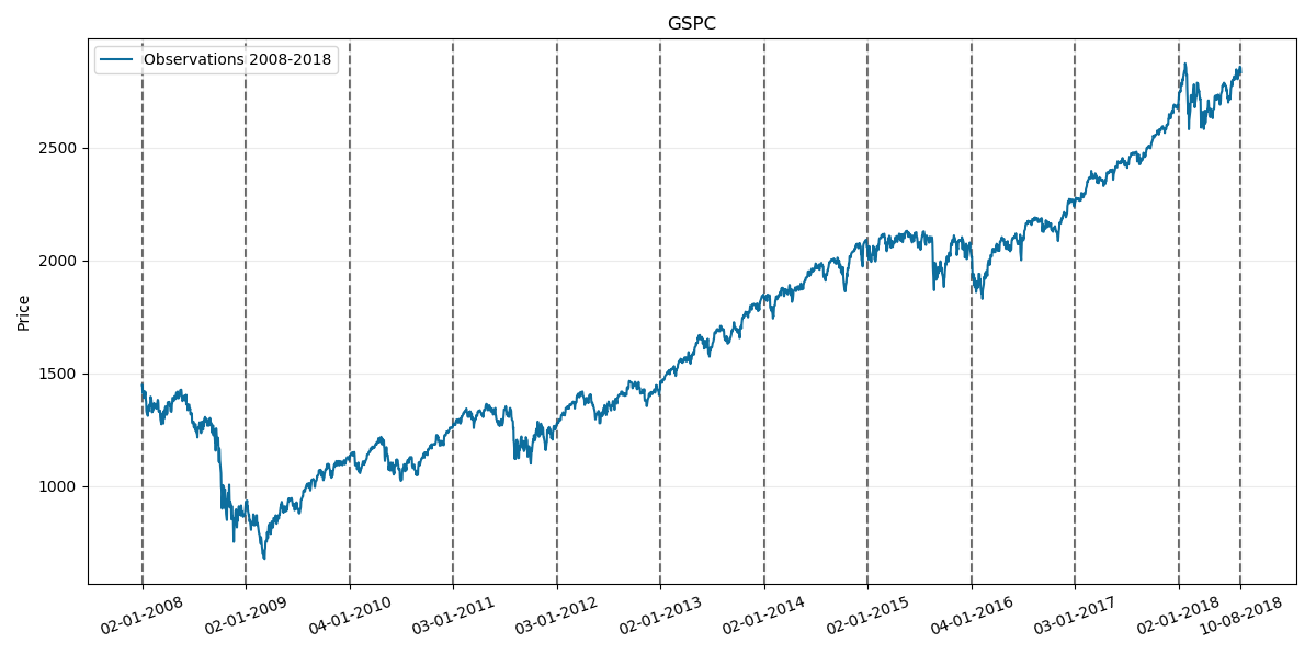
S&P 500 (GSPC)
We will begin with testing our model on GSPC index. Its corresponding prices chart through history is as follows:
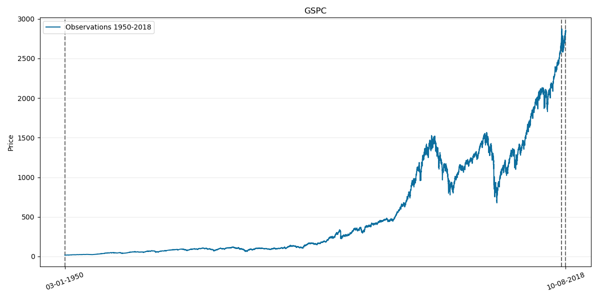
Where the last two vertical lines on the right corresponds to year 2018.
First considered sample period is 2008-2016 so lets take a look at its chart:
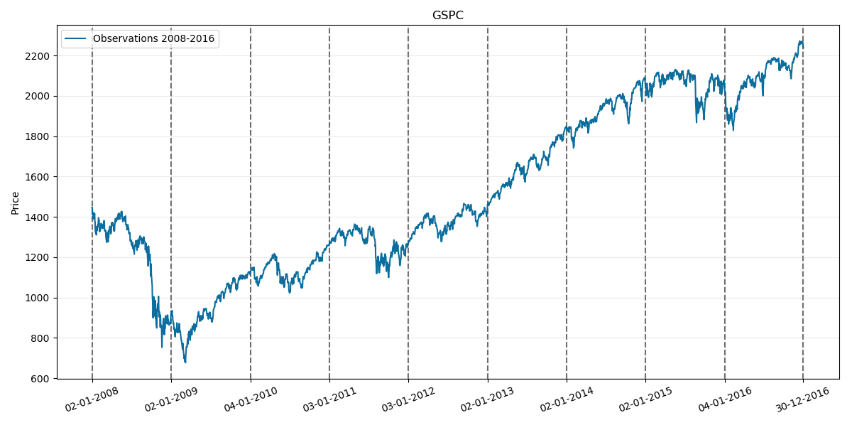
Normalized prices for this period will be respectively:
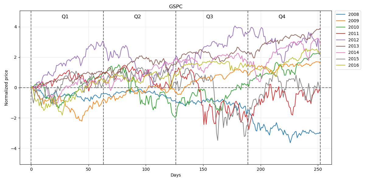
So our prediction for the whole year 2017 with 95% confidence intervals will be:
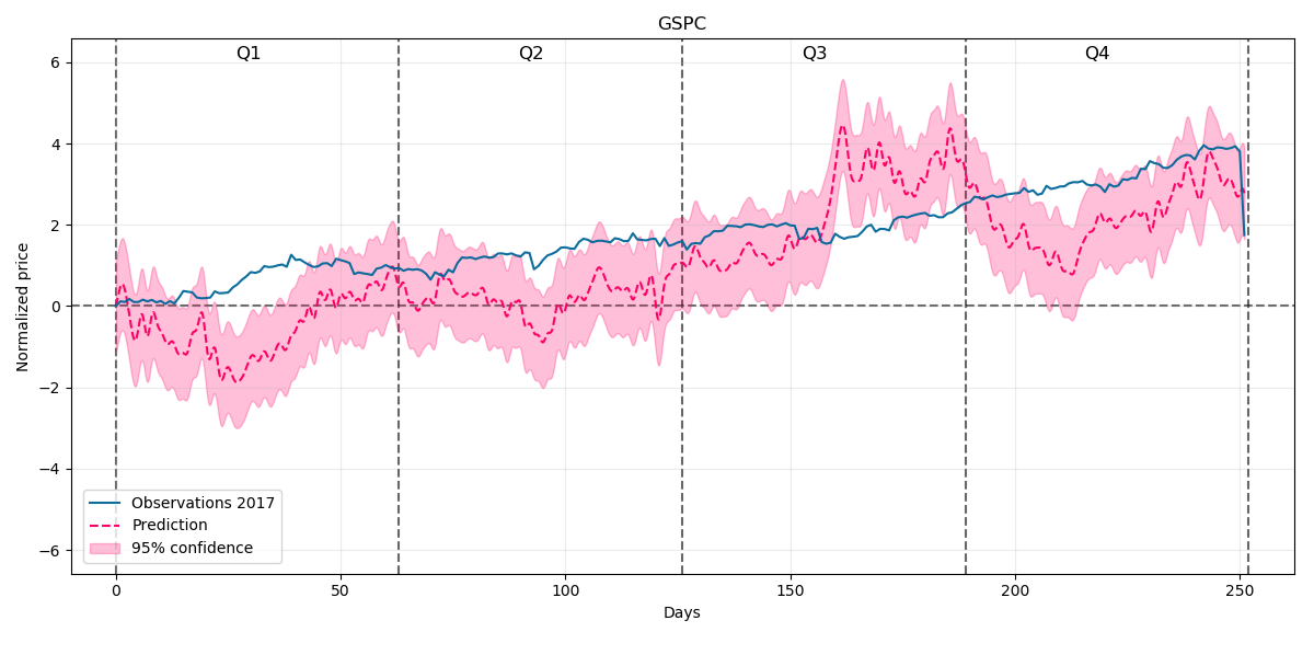
As we can see there are some variations but also the predicted trend for the price is quite good.
Nextly lets consider the 2008-2018 period including first two quarters:
And our prediction for the rest of 2018 will be:
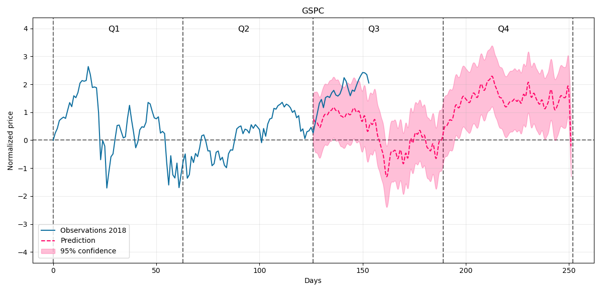
At the beginning prediction drifts away from the price but we can see further some trend going up so it remains for us to wait to the end of the 2018 and compare our forecast with actual price.
The Boeing Company (BA)
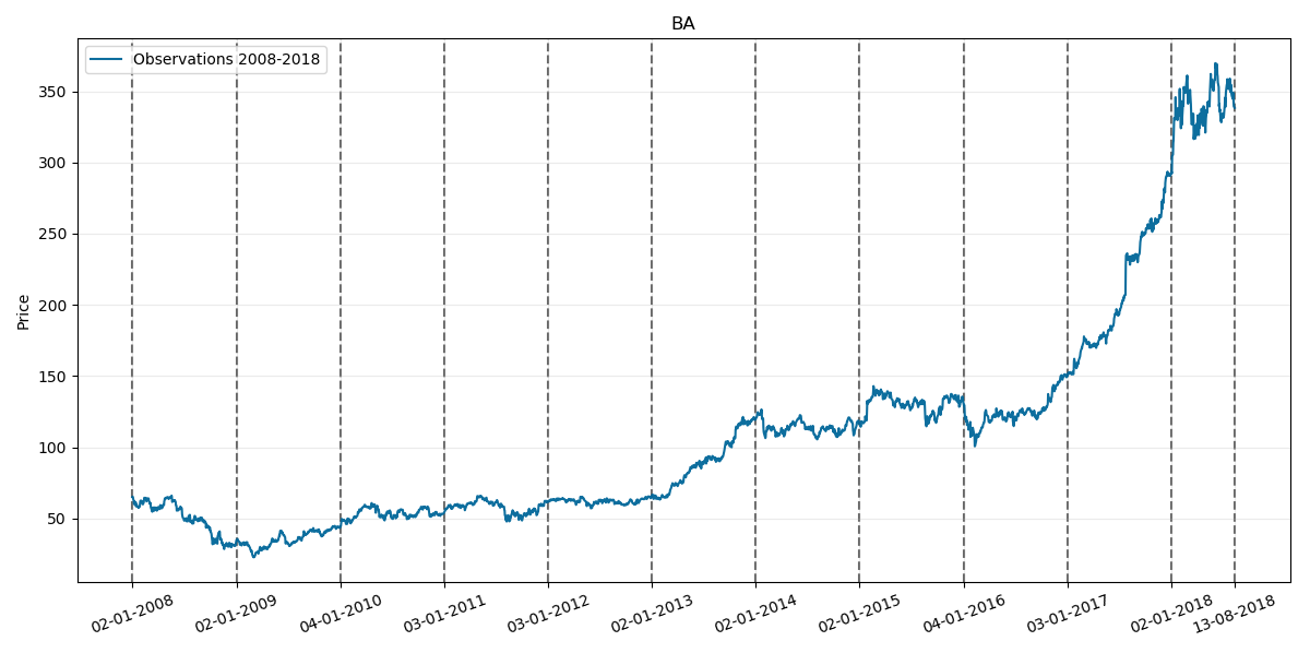
Now lets test our model on BA price. Its corresponding prices chart through history is as follows:
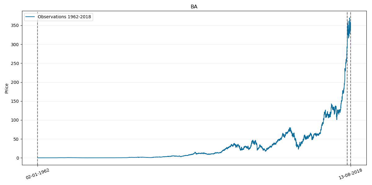
Where the last two vertical lines on the right also corresponds to year 2018.
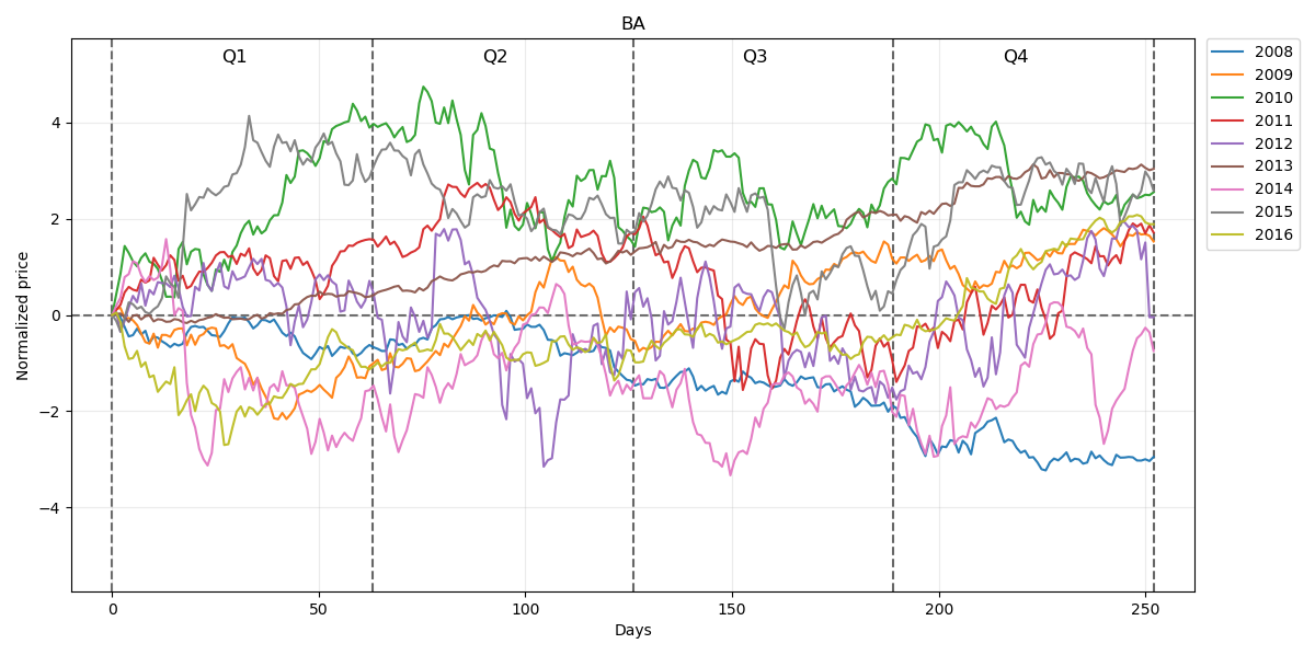
First considered sample period again is 2008-2016 so lets take a look at its chart:
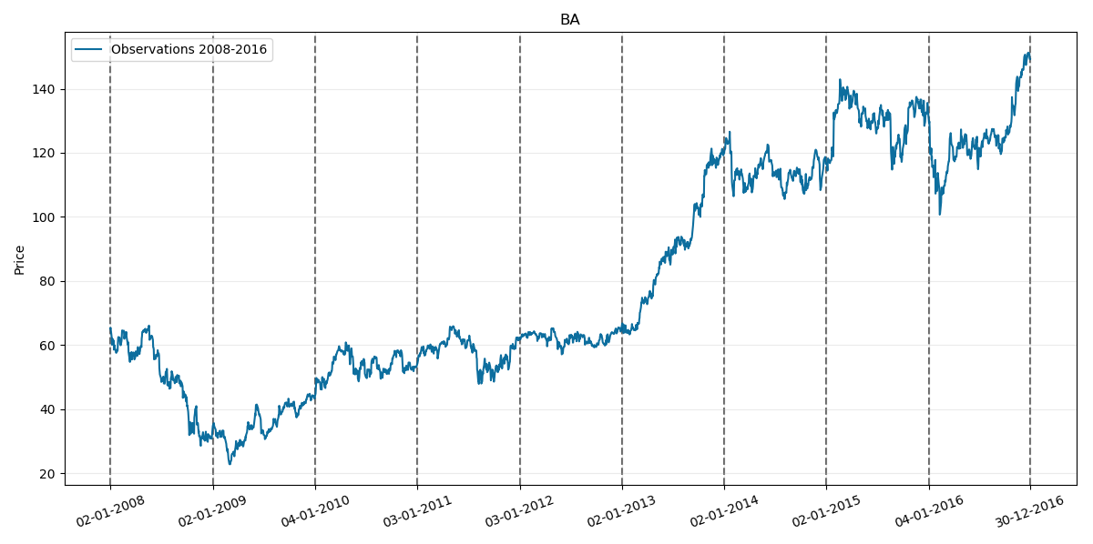
Normalized prices for this period will be respectively:
Our prediction for the whole year 2017 with 95% confidence intervals will be:
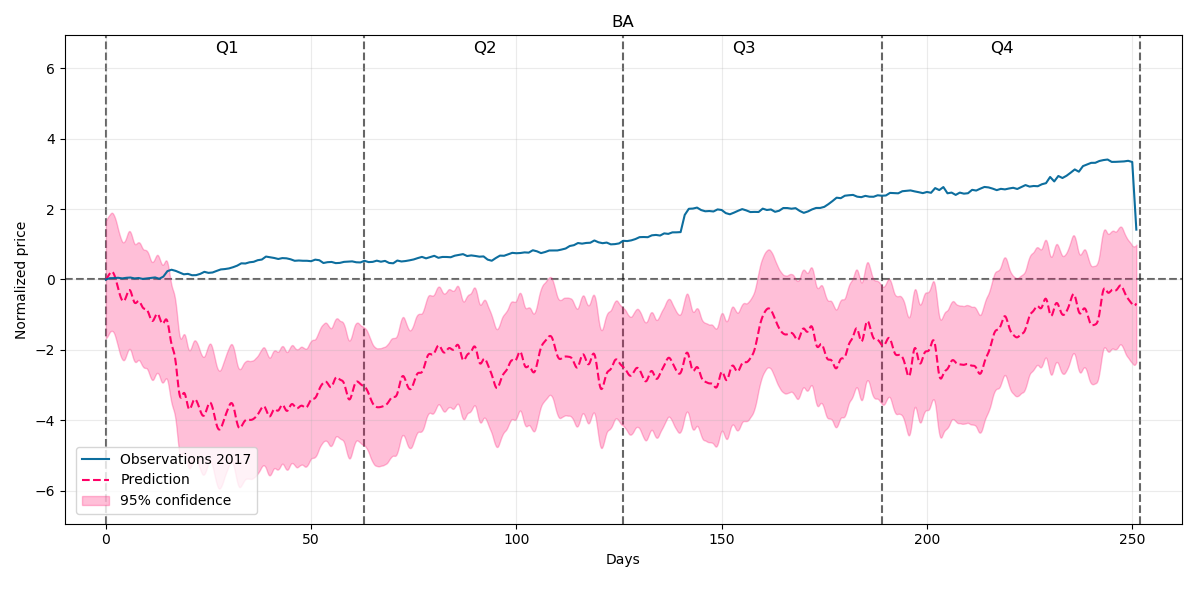
This time our model at the beginning of the year underestimates the price behaviour but later on the trend of the forecast is quite well covering the prices trend direction.
Nextly lets consider the 2008-2018 period including first two quarters:
And our prediction for the rest of 2018 will be:
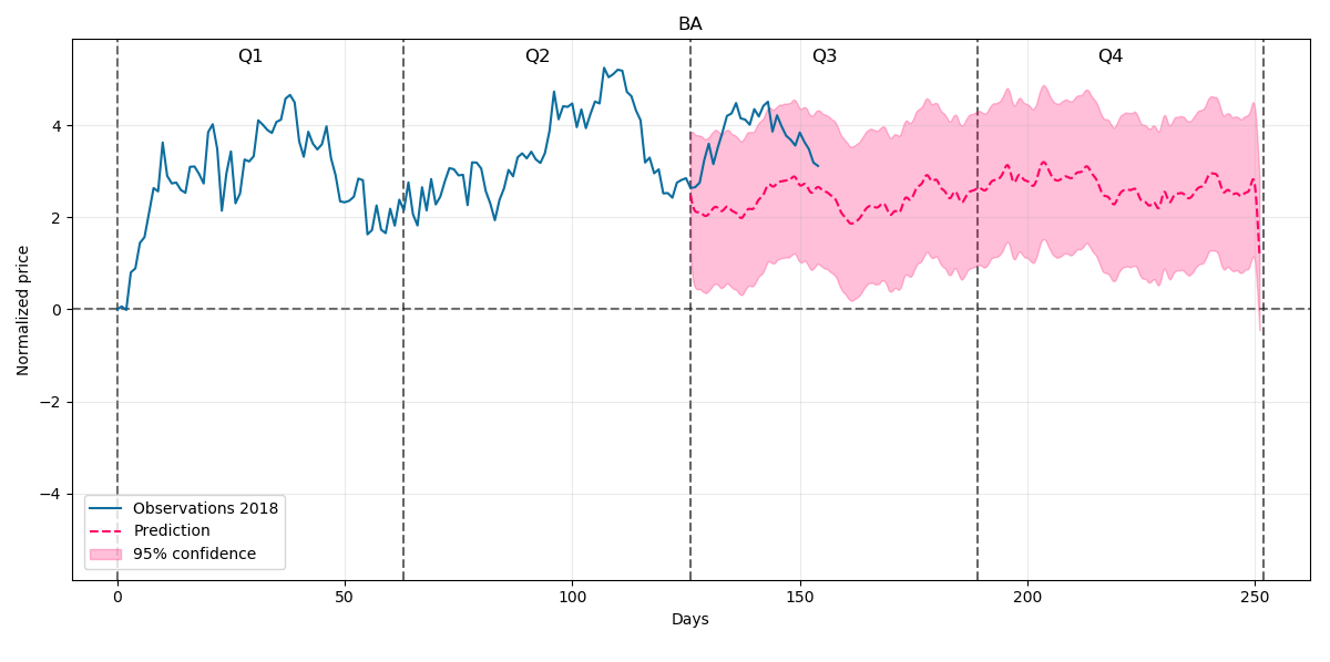
At the beginning the prediction a little bit drifts away from the price but we can see further some stable trend going sideways so the time will verify whether it is a good forecast.
Starbucks (SBUX)
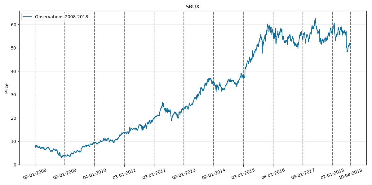
Lastly lets test our model on SBUX. Its corresponding prices chart through history is as follows:
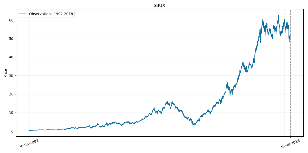
Where the last two vertical lines on the right as usual corresponds to year 2018.
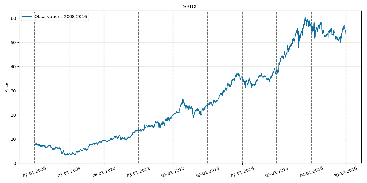
First considered sample period again is 2008-2016 so lets take a look at its chart:
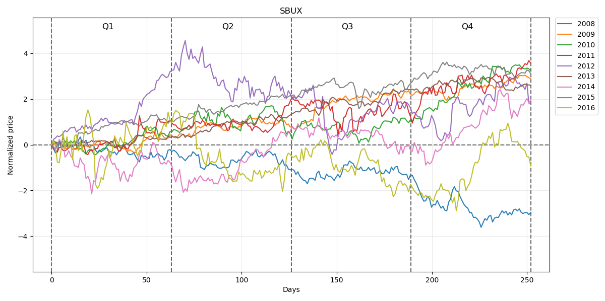
Normalized prices for this period will be respectively:
Our prediction for the whole year 2017 with 95% confidence intervals will be:
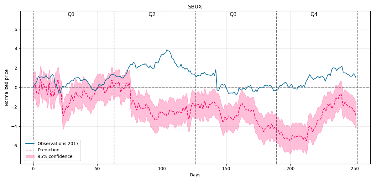
This time our model doesn't forecast as well as previously. There are some good trend prediction in the beginning of the year but nextly it greatly underestimates the behaviour and again in the later period it gets some good forecast, mainly in the last quarter.
Nextly lets consider the 2008-2018 period including first two quarters:
And our prediction for the rest of 2018 will be:
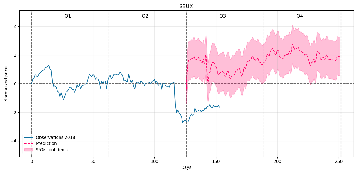
At the beginning the prediction greatly overestimates the behaviour but we can see some stable trend goind upwards from about 150 day further on so it remains again for us to wait and verify what happens next.
Summary
As said earlier the aim of this project was to learn mathematical concepts of GP and implement it later on. We saw that sometimes it forecasted prices trend surprisingly well and sometimes terrible so I wouldn't invest my own money solely relying on GP, but maybe after doing some technical analysis and finding the common results based on analysis and GP I guess why not. Potentially it could be another good technical indicator.
Mathematical definitions and theoretical descriptions were taken from positions listed in bibliography.
Bibliography
- Bengio, Chapados, Forecasting and Trading Commodity Contract Spreads with Gaussian Processes, 2007,
- Correa, Farrell, Gaussian Process Regression Models for Predicting Stock Trends, 2007,
- Chen, Gaussian process regression methods and extensions for stock market prediction, 2017
- Rasmussen, Williams, Gaussian Processes for Machine Learning, 2006