easystats / Modelbased
Programming Languages
modelbased 
modelbased is a lightweight package helping with model-based
estimations, used in the computation of marginal means, contrast
analysis and model predictions.
Installation
Run the following to install the stable release of modelbased from CRAN:
install.packages("modelbased")
Or this one to install the latest development version:
install.packages("remotes")
remotes::install_github("easystats/modelbased")
Documentation
Click on the buttons above to access the package documentation and the easystats blog, and check-out these vignettes:
- Visualisation matrix
- Marginal means
- Contrast analysis
- Use a model to make predictions
- Describe non-linear curves
Features
The package is built around 5 main functions:
-
estimate_means(): Estimates the average values at each factor levels -
estimate_contrasts(): Estimates and tests contrasts between different factor levels -
estimate_slopes(): Estimates the slopes of numeric predictors at different factor levels -
estimate_response(): Predict the response variable using the model -
estimate_smooth(): Describes a non-linear term (e.g. in GAMs) by its linear parts
These functions are powered by the
visualisation_matrix()
function, a smart tool for guessing the appropriate reference grid.
The package currently only supports rstanarm models, but will be
expanded to cover a large variety of frequentist and Bayesian models.
Examples
Create smart grids to represent complex interactions
Check-out this vignette to create this plot:
Estimate marginal means
Check-out this vignette to create this plot:
library(rstanarm)

model <- stan_glm(Sepal.Width ~ Species, data = iris)

estimate_means(model)
## Species    | Mean |       95% CI
## --------------------------------
## setosa     | 3.43 | [3.34, 3.52]
## versicolor | 2.77 | [2.68, 2.87]
## virginica  | 2.97 | [2.89, 3.07]
Contrast analysis
Check-out this vignette to create this plot:
estimate_contrasts(model)
## Level1     |     Level2 | Difference |         95% CI |     pd | % in ROPE | Std_Difference
## -------------------------------------------------------------------------------------------
## setosa     | versicolor |       0.66 | [ 0.53,  0.80] |   100% |        0% |           1.51
## setosa     |  virginica |       0.45 | [ 0.33,  0.59] |   100% |        0% |           1.04
## versicolor |  virginica |      -0.20 | [-0.34, -0.07] | 99.83% |     6.68% |          -0.47
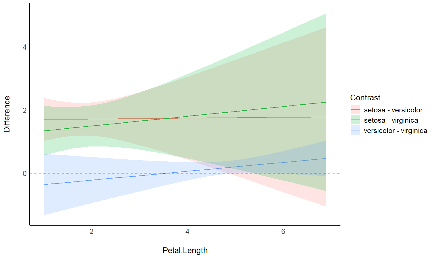
Check the contrasts at different points of another linear predictor
model <- stan_glm(Sepal.Width ~ Species * Petal.Length, data = iris)

estimate_contrasts(model, modulate = "Petal.Length", length = 3)
## Level1     |     Level2 | Petal.Length | Difference |        95% CI |     pd | % in ROPE | Std_Difference
## ---------------------------------------------------------------------------------------------------------
## setosa     | versicolor |         1.00 |       1.67 | [ 1.05, 2.27] |   100% |        0% |           3.84
## setosa     |  virginica |         1.00 |       1.34 | [ 0.59, 2.07] |   100% |     0.02% |           3.07
## versicolor |  virginica |         1.00 |      -0.33 | [-1.27, 0.57] | 75.48% |    13.60% |          -0.76
## setosa     | versicolor |         3.95 |       1.61 | [ 0.66, 2.54] | 99.92% |     0.07% |           3.70
## setosa     |  virginica |         3.95 |       1.66 | [ 0.69, 2.68] | 99.90% |     0.15% |           3.81
## versicolor |  virginica |         3.95 |       0.05 | [-0.23, 0.34] | 63.50% |    47.48% |           0.12
## setosa     | versicolor |         6.90 |       1.54 | [-0.54, 3.60] | 93.00% |     2.73% |           3.54
## setosa     |  virginica |         6.90 |       2.00 | [-0.02, 4.00] | 97.35% |     1.27% |           4.58
## versicolor |  virginica |         6.90 |       0.44 | [-0.08, 0.96] | 94.62% |     8.80% |           1.01
Find a predictor’s slopes at each factor level
estimate_slopes(model)
## Species    | Median |        95% CI |     pd | % in ROPE | Std. Median
## ----------------------------------------------------------------------
## setosa     |   0.34 | [-0.05, 0.69] | 96.00% |     8.48% |        1.37
## versicolor |   0.36 | [ 0.18, 0.54] | 99.98% |     0.18% |        1.46
## virginica  |   0.23 | [ 0.07, 0.38] | 99.88% |     5.78% |        0.93
Generate predictions from your model to compare it with original data
Check-out this vignette to create this plot:
estimate_response(model)
| Sepal.Length | Species | Predicted | CI_low | CI_high |
|---|---|---|---|---|
| 5.1 | setosa | 1.47 | 0.98 | 1.98 |
| 4.9 | setosa | 1.45 | 0.92 | 1.97 |
| 4.7 | setosa | 1.41 | 0.88 | 1.96 |
| 4.6 | setosa | 1.42 | 0.92 | 1.98 |
| 5.0 | setosa | 1.46 | 0.90 | 1.96 |
| 5.4 | setosa | 1.51 | 1.00 | 2.11 |
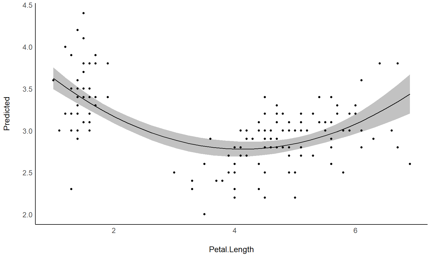
Estimate the link between the response and a predictor
See this
vignette
to create this plot:

model <- stan_glm(Sepal.Width ~ poly(Petal.Length, 2), data = iris)

estimate_link(model)
| Petal.Length | Predicted | CI_low | CI_high |
|---|---|---|---|
| 1.00 | 3.62 | 3.49 | 3.75 |
| 1.98 | 3.18 | 3.09 | 3.26 |
| 2.97 | 2.90 | 2.81 | 2.99 |
| 3.95 | 2.78 | 2.69 | 2.87 |
| 4.93 | 2.83 | 2.77 | 2.91 |
| 5.92 | 3.05 | 2.94 | 3.16 |
| 6.90 | 3.44 | 3.20 | 3.68 |
Describe the smooth term by its linear parts
estimate_smooth(model)
## Part | Start |  End |   Size | Trend | Linearity
## ------------------------------------------------
## 1    |  1.00 | 3.62 | 50.00% | -0.19 |      0.96
## 2    |  3.62 | 6.90 | 50.00% |  0.08 |      0.81


