lambdaclass / Options_backtester
Projects that are alternatives of or similar to Options backtester
Options Backtester
Simple backtester to evaluate and analyse options strategies over historical price data.
Requirements
- Python >= 3.6
- pipenv
Setup
Install pipenv
$> pip install pipenv
Create environment and download dependencies
$> make install
Activate environment
$> make env
Run Jupyter notebook
$> make notebook
Run tests
$> make test
Usage
Sample backtest
You can run this example by putting the code into a Jupyter Notebook/Lab file in this directory.
import os
import sys

BACKTESTER_DIR = os.getcwd()
TEST_DATA_DIR = os.path.join(BACKTESTER_DIR, 'backtester', 'test', 'test_data')
SAMPLE_STOCK_DATA = os.path.join(TEST_DATA_DIR, 'test_data_stocks.csv')
SAMPLE_OPTIONS_DATA = os.path.join(TEST_DATA_DIR, 'test_data_options.csv')
from backtester import Backtest, Stock, Type, Direction
from backtester.datahandler import HistoricalOptionsData, TiingoData
from backtester.strategy import Strategy, StrategyLeg
First we construct an options datahandler.
options_data = HistoricalOptionsData(SAMPLE_OPTIONS_DATA)
options_schema = options_data.schema
Next, we'll create a toy options strategy. It will simply buy a call and a put with dte between $80$ and $52$ and exit them a month later.
sample_strategy = Strategy(options_schema)

leg1 = StrategyLeg('leg_1', options_schema, option_type=Type.CALL, direction=Direction.BUY)
leg1.entry_filter = (options_schema.dte < 80) & (options_schema.dte > 52)

leg1.exit_filter = (options_schema.dte <= 52)

leg2 = StrategyLeg('leg_2', options_schema, option_type=Type.PUT, direction=Direction.BUY)
leg2.entry_filter = (options_schema.dte < 80) & (options_schema.dte > 52)

leg2.exit_filter = (options_schema.dte <= 52)

sample_strategy.add_legs([leg1, leg2]);
We do the same for stocks: create a datahandler together with a list of the stocks we want in our inventory and their corresponding weights. In this case, we will hold VOO, TUR and RSX, with $0.4$, $0.1$ and $0.5$ weights respectively.
stocks_data = TiingoData(SAMPLE_STOCK_DATA)
stocks = [Stock('VOO', 0.4), Stock('TUR', 0.1), Stock('RSX', 0.5)]
We set our portfolio allocation, i.e. how much of our capital will be invested in stocks, options and cash. We'll allocate 50% of our capital to stocks and the rest to options.
allocation = {'stocks': 0.5, 'options': 0.5, 'cash': 0.0}
Finally, we create the Backtest object.
bt = Backtest(allocation, initial_capital=1_000_000)

bt.stocks = stocks
bt.stocks_data = stocks_data

bt.options_strategy = sample_strategy
bt.options_data = options_data
And run the backtest with a rebalancing period of one month.
bt.run(rebalance_freq=1)
0% [██████████████████████████████] 100% | ETA: 00:00:00
Total time elapsed: 00:00:00
| leg_1 | leg_2 | totals | |||||||||||||||
|---|---|---|---|---|---|---|---|---|---|---|---|---|---|---|---|---|---|
| contract | underlying | expiration | type | strike | cost | order | contract | underlying | expiration | type | strike | cost | order | cost | qty | date | |
| 0 | SPX170317C00300000 | SPX | 2017-03-17 | call | 300 | 195010.0 | Order.BTO | SPX170317P00300000 | SPX | 2017-03-17 | put | 300 | 5.0 | Order.BTO | 195015.0 | 2.0 | 2017-01-03 |
| 1 | SPX170317C00300000 | SPX | 2017-03-17 | call | 300 | -197060.0 | Order.STC | SPX170317P00300000 | SPX | 2017-03-17 | put | 300 | -0.0 | Order.STC | -197060.0 | 2.0 | 2017-02-01 |
| 2 | SPX170421C00500000 | SPX | 2017-04-21 | call | 500 | 177260.0 | Order.BTO | SPX170421P01375000 | SPX | 2017-04-21 | put | 1375 | 60.0 | Order.BTO | 177320.0 | 2.0 | 2017-02-01 |
| 3 | SPX170421C00500000 | SPX | 2017-04-21 | call | 500 | -188980.0 | Order.STC | SPX170421P01375000 | SPX | 2017-04-21 | put | 1375 | -5.0 | Order.STC | -188985.0 | 2.0 | 2017-03-01 |
| 4 | SPX170519C01000000 | SPX | 2017-05-19 | call | 1000 | 138940.0 | Order.BTO | SPX170519P01650000 | SPX | 2017-05-19 | put | 1650 | 100.0 | Order.BTO | 139040.0 | 3.0 | 2017-03-01 |
| 5 | SPX170519C01000000 | SPX | 2017-05-19 | call | 1000 | -135290.0 | Order.STC | SPX170519P01650000 | SPX | 2017-05-19 | put | 1650 | -20.0 | Order.STC | -135310.0 | 3.0 | 2017-04-03 |
The trade log (bt.trade_log) shows we executed 6 trades: we bought one call and one put on 2017-01-03, 2017-02-01 and 2017-03-01, and exited those positions on 2017-02-01, 2017-03-01 and 2017-04-03 respectively.
The balance data structure shows how our positions evolved over time:
- We started with $1000000 on 2017-01-02
-
total capitalis the sum ofcash,stocks capitalandoptions capital -
% changeshows the inter day change intotal capital -
accumulated returngives the compounded return intotal capitalsince the start of the backtest
bt.balance.head()
| total capital | cash | VOO | TUR | RSX | options qty | calls capital | puts capital | stocks qty | VOO qty | TUR qty | RSX qty | options capital | stocks capital | % change | accumulated return | |
|---|---|---|---|---|---|---|---|---|---|---|---|---|---|---|---|---|
| 2017-01-02 | 1.000000e+06 | 1000000.00000 | NaN | NaN | NaN | NaN | NaN | NaN | NaN | NaN | NaN | NaN | 0.0 | 0.000000 | NaN | NaN |
| 2017-01-03 | 9.990300e+05 | 110117.40592 | 199872.763320 | 49993.281167 | 249986.549593 | 2.0 | 389060.0 | 0.0 | 16186.0 | 1025.0 | 1758.0 | 13403.0 | 389060.0 | 499852.594080 | -0.000970 | 0.999030 |
| 2017-01-04 | 1.004228e+06 | 110117.40592 | 201052.238851 | 50072.862958 | 251605.333911 | 2.0 | 391380.0 | 0.0 | 16186.0 | 1025.0 | 1758.0 | 13403.0 | 391380.0 | 502730.435720 | 0.005203 | 1.004228 |
| 2017-01-05 | 1.002706e+06 | 110117.40592 | 200897.553535 | 49865.950301 | 250564.686850 | 2.0 | 391260.0 | 0.0 | 16186.0 | 1025.0 | 1758.0 | 13403.0 | 391260.0 | 501328.190686 | -0.001516 | 1.002706 |
| 2017-01-06 | 1.003201e+06 | 110117.40592 | 201680.647945 | 49372.543196 | 248830.275081 | 2.0 | 393200.0 | 0.0 | 16186.0 | 1025.0 | 1758.0 | 13403.0 | 393200.0 | 499883.466222 | 0.000494 | 1.003201 |
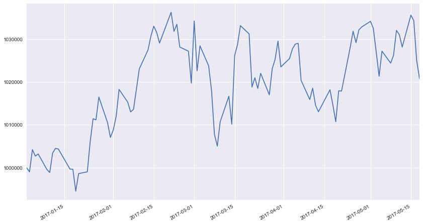
Evolution of our total capital over time:
bt.balance['total capital'].plot();
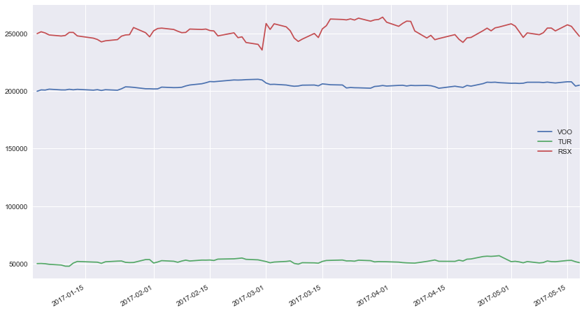
Evolution of our stock positions over time:
bt.balance[[stock.symbol for stock in stocks]].plot();
More plots and statistics are available in the backtester.statistics module.
Other strategies
The Strategy and StrategyLeg classes allow for more complex strategies; for instance, a long strangle could be implemented like so:
# Long strangle
leg_1 = StrategyLeg('leg_1', options_schema, option_type=Type.PUT, direction=Direction.BUY)
leg_1.entry_filter = (options_schema.underlying == 'SPX') & (options_schema.dte >= 60) & (options_schema.underlying_last <= 1.1 * options_schema.strike)
leg_1.exit_filter = (options_schema.dte <= 30)

leg_2 = StrategyLeg('leg_2', options_schema, option_type=Type.CALL, direction=Direction.BUY)
leg_2.entry_filter = (options_schema.underlying == 'SPX') & (options_schema.dte >= 60) & (options_schema.underlying_last >= 0.9 * options_schema.strike)
leg_2.exit_filter = (options_schema.dte <= 30)

strategy = Strategy(options_schema)
strategy.add_legs([leg_1, leg_2]);
You can explore more usage examples in the Jupyter notebooks.
Recommended reading
For complete novices in finance and economics, this post gives a comprehensive introduction.
Books
Introductory
- Option Volatility and Pricing 2nd Ed. - Natemberg, 2014
- Options, Futures, and Other Derivatives 10th Ed. - Hull 2017
- Trading Options Greeks: How Time, Volatility, and Other Pricing Factors Drive Profits 2nd Ed. - Passarelli 2012
Intermediate
- Trading Volatility - Bennet 2014
- Volatility Trading 2nd Ed. - Sinclair 2013
Advanced
- Dynamic Hedging - Taleb 1997
- The Volatility Surface: A Practitioner's Guide - Gatheral 2006
- The Volatility Smile - Derman & Miller 2016
Papers
- Volatility: A New Return Driver?
- Easy Volatility Investing
- Everybody’s Doing It: Short Volatility Strategies and Shadow Financial Insurers
- Volatility-of-Volatility Risk
- The Distribution of Returns
- Safe Haven Investing Part I - Not all risk mitigation is created equal
- Safe Haven Investing Part II - Not all risk is created equal
- Safe Haven Investing Part III - Those wonderful tenbaggers
- Insurance makes wealth grow faster
- Ergodicity economics
- The Rate of Return on Everything, 1870–2015
- Volatility and the Alchemy of Risk


