martin-pr / Possumwood

A simple OpenGL demo

A simple demo showing how to load an .obj file (positions, normals and topology) and display it using OpenGL.

Named vertex attributes p and n are loaded from an .obj file, and passed through to an OpenGL vertex/fragment shader setup. In later demos, this setup is wrapped-up in a subnetwork.

Automatic normals

When an mesh file doesn't include explicit normals, it is relatively easy to use a fragment shader to "autogenerate" normals using screen-space derivatives dFdx() and dFdy(). This demo shows how to do that in Possumwood - just have a look at fragment_shared source.

Turntable demo

A simple shader setup passing a time value (i.e., the timeline value) as a uniform into the shader (together with viewport parameters). This value is then converted in the vertex_shader to a transformation matrix used to rotate a model.

Wireframe using a geometry shader

Wireframe mode is one of the rendering modes of OpenGL. A similar but more controllable effect can be achieved by processing a model using a geometry shader, which allows to convert primitives to a different number of primitives of the same or different type.

This setup shows how to emit a line for each polygon edge of the input geometry using a program in geometry_shader. It also shows how to adjust the line width to screen resolution, maintaining the width independent to view parameters.

Mesh subdivision in a geometry shader

While modern GPUs contain a bespoke functionality for subdivision, this simple demo shows how a similar (if limited) effect can be achieved using a simple geometry shader.

This demo implements a simple interpolative sudvision scheme with normal-based displacement. All subdivision computation is done in a geometry shader, with additional vertices and topology emitted by calling a recusive function. This approach is just a toy example, as it is strictly limited by the capabilities of individual GPUs - in practical applications, bespoke tesselation shaders perform much better.

PN Triangles in a geometry shader

Curved PN Triangles is a simple geometry subdivision scheme, replacing all triangles with a bezier patch directly on the GPU. The shape interpolation uses a cubic spline, and normals are interpolated using a quadratic spline to maintain continuity.

This implementation uses a geometry shader for emitting additional polygons.

_{Vlachos, Alex, et al. "Curved PN triangles." Proceedings of the 2001 symposium on Interactive 3D graphics. ACM, 2001.}

Infinite ground plane

A simple way of generating procedural graphics using GLSL employs rendering a single polygon covering the whole frame, and a per-pixel fragment shader (with additional inputs) to compute the final colour. A number of examples of this approach can be found at ShaderToy.

This demo is a simple example of such approach - based on a ray generated from a near and far plane point corresponding to a screen pixel, it computes the position of ray's intersection with the ground plane (y==0), and uses this information to synthesize an "infinite" ground plane covered in checkerboard, with a "spotlight". The fragment shader does all the computation - from ray intersection, through colour and checkerboard generation, to depth-value computation to allow the ground plane to composit correctly with other objects in a scene.

Shadertoy

ShaderToy is a community of artists and programmers centered around generating interesting graphics content in GLSL using a single fragment shader.

One of the common techniques to generate procedural 3D content in a fragment shader is Raymarching - a simple method of tracing rays against shapes represented as Signed Distance Functions, and generating 3D content based on them.

This demo is a port of a ShaderToy demo by Indigo Quilezles, showing different SDFs and a few additional effects that can be achieved by raymarching. A comprehensive raymarching tutorial can be found at the RaymarchingWorkshop.

Skybox

A classical way of generating sky and background in games is to render a cube or spherical map on the far plane (behind all other objects). This method is called CubeMap, SkyBox or SkyDome.

This simple demo shows this technique on a spherical texture from HDRI Haven.

Reflection mapping

Reflection mapping is a simple image-based lighting technique for simulating purely reflective materials. It only behaves correcty for convex shapes, but even with this strict limitation, it has been long established as a simple method for reflective surfaces in computer graphics.

This demo combines a skybox with a "purely reflective" material.

Gourand shading

Gourand shading is one of the simplest method of polygonal mesh shading. It computes colour by linearly interpolating vertex colours in screen space, making it cheap but less physically accurate than Phong or physics-based shading methods.

This demo combines Gourand shading with Phong reflection model, reproducing an old "fixed-pipeline" shading model of OpenGL.

Phong shading

Phong shading computes lighting of a surface by interpolating per-pixel surface normal. Compared to Gourand shading, this method leads to smoother and more realistic surface looks better describing the shape of the object, and significantly more accurate high-frequency components computation (i.e., specular component in the Phong lighting model).

This demo implements Phong shading with a Phong reflection model and a single point light source. The setup is wrapped in a subnetwork - just double-click the blue node to "enter" it.

Material capture shader

MatCap or LitSphere is a simple technique for representing the properties of both the material and the environment light in a single texture. By "baking in" the two dimensions of BRDF representing incoming light, MatCap determines the final colour solely by using the difference vector between the view ray and the surface normal.

This simple approach can yield surprisingly realistic results, and has been used in games, scultping software and for capturing and representing artistic styles.

_{Sloan, Peter-Pike J., et al. "The lit sphere: A model for capturing NPR shading from art." Graphics interface. Vol. 2001. 2001.}

Normal mapping

Normal mapping is a simple method for adding texture-based geometry details to a coarse model. It uses a texture to represent normal perturbation that would result from a significantly more detail in the surface mesh, without having to represent that detail explicitly in the underlying geometry. In games, this technique is often used to represent a complex model with all its detail, without having to explicitly store a heavy geometry.

This simple demo demonstrates a combination of normal mapping implemented in a fragment shader, together with displacement mapping implemented as a geometry shader. The lighting is implemented as a simple single light-source Phong reflection model.

_{Blinn, James F. "Simulation of wrinkled surfaces." ACM SIGGRAPH computer graphics. Vol. 12. No. 3. ACM, 1978. Mikkelsen, Morten. "Simulation of wrinkled surfaces revisited." (2008).}

SDF-based text rendering

Rendering text in OpenGL is usually implemented using a simple texture. However, such text "pixelates" when viewed up-close. A simple method to improve on its appearance uses a Signed distance function to represent letter boundaries - by exploiting the interpolation abilities of GPU hardware, it is possible to represent a text boundary with significantly more precision by using the directional information represented in SDF texture differential.

This demo shows a simple implementation of this technique.

_{Green, Chris. "Improved alpha-tested magnification for vector textures and special effects." ACM SIGGRAPH 2007 courses. ACM, 2007.}

OBJ file loading

This simple demo shows how to load an object from .obj file, and display it in the viewport.

The display code is contained in a subnetwork (double click the blue node to "enter" it), and is based on a trivial implementation of a vertex and fragment OpenGL shader.

Lua mesh generation

A simple setup demonstrating a way to generate a new mesh in Lua using simple mesh bindings, and display the result using OpenGL. The main functionality is contained within the script node, which functions in the environment constructed by its inputs, and produces a state with new values on its output. The mesh extract node then extracts a mesh from the state and feeds it into CGAL mesh display node.

CGAL normals generation

To display a polygonal mesh on a GPU, the model needs to contain surface-normal information for shading. While this information can be auto-generated, an explicitly represented normal can improve surface properties like smoothness or shape details.

This simple demo shows two methods of computing normals using the CGAL library.

CGAL mesh decimation

Mesh simplification (decimation) is a common operation in mesh processing - it aims to reduce the mesh complexity without removing its details, reducing the memory footprint without compromising the quality of the resulting model.

This demo shows how to use CGAL's implementation of mesh decimation in Possumwood, allowing to experiment with its various parameters.

Mesh Subdivision in CGAL

This simple demo demonstrates the mesh subdivision functionality as implemented in CGAL.

There are four subdivision methods implemented in CGAL - Catmull Clark, Loop, Doo Sabin and Sqrt 3. In Possumwood, all these are implemented as a single node acting on the polyhedron type.

CSG in CGAL

CGAL implements CSG (Constructive Solid Geometry) through Nef Polyhedra, a boundary-representation datastructure that is closed under Boolean set of operations.

This demo shows how a simple CSG setup can be created in Possumwood. A subnetwork is used to generate a sphere through Lua scripting, and convert it to a Nef polyhedron. This is then used as an input to CSG Boolean operations, result of which is displayed using a conversion to standard CGAL Polyhedron and an OpenGL setup in a subnetwork.

Minkowski addition in CGAL

Minkowski addition allows to combine two polyhedra such that the result is a polyhedron where one of the object has been "swiped" around the other (please see the link for more accurate description).

In CGAL, Minowski addition is implemented on top of the Nef polyhedra. This example setup shows how Minkowski addition can be used to "expand" and "round edges" a polyhedron.

Convex Hull in CGAL

Convex hull algorithm, implemented in CGAL, generates the smallest possible convex polyhedron fully enclosing a set of points. In Possumwood, the input to convex hull is a set of points from input meshes, and output is a convex polyhedron enclosing all of them.

Convex hull is useful for mesh generation for 3D printing - alongside boolean operations, it allows for creating complex shapes out of very simple primitives.

Face selection in CGAL

Selection in CGAL's mesh processing is primarily used to determine which region is supposed to be influenced by an operation.

This demo shows the most basic selection by mesh intersection - faces of a mesh within another mesh are selected, and displayed in a different color.

Face selection in CGAL

Selection in CGAL's mesh processing is primarily used to determine which region is supposed to be influenced by an operation.

This demo shows "boolean" set operations on selections, allowing to procedurally create more complex selections from simple inputs.

Isotropic remeshing in CGAL

Isotropic remeshing alters the input mesh such that it consists of "well behaved" polygons - uniformly distributes polygons with similar area and edge lengths.

This demo shows how to use remeshing of whole meshes in Possumwood. The input for remeshing is a selection - it is also possible to remesh only a part of the input mesh.

Botsch, Mario, and Leif Kobbelt. "A remeshing approach to multiresolution modeling." Proceedings of the 2004 Eurographics/ACM SIGGRAPH symposium on Geometry processing. 2004.

Lua addition node

This simple demo shows how to create a subnetwork performing simple addition (and exposing input parameters) with a simple Lua script.

Double click the node too see its content.

Lua multiplication node

This simple demo shows how to create a subnetwork performing simple multiplication (and exposing input parameters) with a simple Lua script.

Double click the node too see its content.

Animated cube

A simple demo showing how to use a Lua script to create animated data, which are then fed as an input to a vector input of the cube node, animating its position.

Lua-based image synthesis

Possumwood contains a simple integration of the Lua scripting language, allowing to manipulate in-scene objects using code contained in nodes.

This demo shows how to synthesize an image programatically. It "injects" the images plugin into the input Lua context (i.e., the environment for running a script), and generates an image, which is then extracted from the output state using an image extract node. The result is then passed on an image-display subnetwork.

Lua expression-based image synthesis

This demo builds on the Lua Grid setup, extending it by additional parameters, and wrapping it in a subnetwork (double click any blue nodes to "enter" them).

Lua image tonemapping

Lua expressions in Possumwood can be also used to manipulate HDR images.

This demo shows how to implement simple Gamma compression tonemapping operator in Lua, and how to wrap it into a subnetwork with exposed parameters. Possumwood allows arbitrary nesting of nodes in this way, allowing to abstract-away any unnecessary complexity into simple nodes with clean interfaces.

OpenCV image loading and display

This simple demo shows how to load an image using OpenCV's imread() method, and pass the resulting image data to OpenGL as a texture and a set of additional metadata represented by GLSL uniforms.

In following demos, this OpenGL setup is wrapped in a subnetwork.

Image loading

A simple demo showing how to load an image from a file, and display it using an OpenGL setup (wrapped in a subnetwork - enter it by double-clicking the blue node).

Fullscreen image display

While Possumwood's viewport is primarily intended for viewing 3D content, using a set of shaders it is possible to alter it to display 2D textures as well.

This demo uses shaders that ignore the perspective projection matrix and draw 2D image in a 2D front-facing view in the viewport.

Grayscale conversion

Color conversion in OpenCV is implemented in the cvtColor() function. This demo shows how to use the corresponding color node to first convert to grayscale, and then back to BGR to allow the image to be passed to OpenGL as RGB data.

Face detection using Haar cascades

This demo follows the OpenCV's Haar Cascade tutorial - it allows to load a Haar Cascade .xml file in OpenCV's format, use it to detect faces in the input image, and then draw the result into the source image for display.

Lienhart, Rainer, and Jochen Maydt. "An extended set of haar-like features for rapid object detection." Proceedings. international conference on image processing. Vol. 1. IEEE, 2002.

Grayscale image denoising

This tutorial closely follows the OpenCV's denoising tutorial for grayscale images, removing the noise using the non-local means algorithm.

Color image denoising

This tutorial closely follows the OpenCV's denoising tutorial for color images, removing the noise using the non-local means algorithm.

Visualising luminance noise

This tutorial follows the OpenCV's denoising tutorial for grayscale images, but at the end of the processing it subtracts the denoised image from the original (leaving only extracted noise), and equalises the result using cv::equalizeHist() to show the noise structure.

Visualising color noise

This tutorial follows the OpenCV's denoising tutorial for color images, but at the end of the processing it subtracts the denoised image from the original (leaving only extracted noise), and equalises the result using cv::equalizeHist() to show the noise structure.

Discrete Fourier Transform and a simple low-pass filter

The Discrete Fourier Transform (implemented in OpenCV) converts a signal (image) into its complex frequency spectrum. By manipulating the spectrum, it is possible to implement simple frequency filters.

This demo shows how to perform a DFT on an image, and implements a simple frequency cutoff low-pass filter, showing both the image before and after applying this filter.

Video frames

OpenCV's VideoCapture object can be used to extract frames from a video file. This demo shows how to use a video_frame source together with a frame input to link the viewport timeline with a displayed video frame.

Dense optical flow

OpenCV provides a method to compute dense optical flow in the calcOpticalFlowFarneback() function, allowing to detect moving objects in frames without explicitly detecting feature points first.

This demo shows how to set up this type of optical flow in Possumwood, and how to display its results as colours on top of a grayscale animated image.

_{Farnebäck, Gunnar. "Two-frame motion estimation based on polynomial expansion." Scandinavian conference on Image analysis. Springer, Berlin, Heidelberg, 2003.}

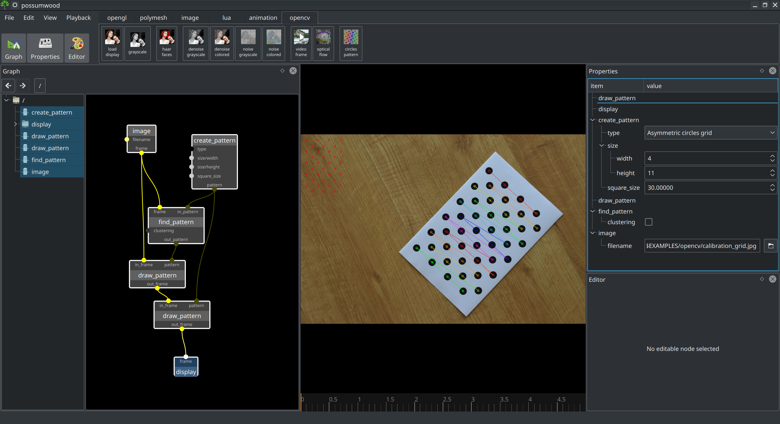
Calibration pattern detection (circles)

Pattern detection is the first step of camera calibration for many computer vision algorithms. This demo shows how a pattern build of circles can be detected using Hough transformation, and assembled into a grid for the use of camera intrinsic and extrinsic calibration.

Calibration pattern detection (chessboard)

Pattern detection is the first step of camera calibration for many computer vision algorithms. This demo shows how a chessboard pattern can be detected using corners feature detection, and assembled into a grid for the use of camera intrinsic and extrinsic calibration.

Camera calibration

The calibration of a camera's intrinsic parameters is an important step for most algorithms in machine vision.

This demo shows how to perform multi-image intrinsic camera calibration using a chessboard pattern, and how to use the solved parameters to undistort an image. This functionality is fully built using OpenCV's functions, wrapped in a set of Possumwood nodes.

The left side of the graph detects a pattern in a set of 4 images, accumulating the results in a points array; the calibrate_camera node computes the intrinsic calibration from a set of input sample points; the undistort node then uses the resulting calibration to correct the distortion of an input image.

Image inpainting using Fast Marching

Image inpainting is an image reconstruction technique, allowing to fill-in missing parts of an image based on existing pixels.

Telea's algorithm shown in this demo uses a Fast Marching method to inpaint pixels from a boundary based on surrounding pixels and boundary's normal direction.

_{Telea, Alexandru. "An image inpainting technique based on the fast marching method." Journal of graphics tools 9.1 (2004): 23-34.}

Image inpainting using Fast Marching

Image inpainting is an image reconstruction technique, allowing to fill-in missing parts of an image based on existing pixels.

The Navier-Stokes-based algorithm shown in this demo uses a heuristic based on fluid dynamics to inpaint a large region of dark pixels in an image, obtained by image thresholding.

_{Bertalmio, Marcelo, Andrea L. Bertozzi, and Guillermo Sapiro. "Navier-stokes, fluid dynamics, and image and video inpainting." Proceedings of the 2001 IEEE Computer Society Conference on Computer Vision and Pattern Recognition. CVPR 2001. Vol. 1. IEEE, 2001.}

Inpainting for image restoration

Image inpainting can be also used to attempt to restore an image where a large portion of the original data is missing.

This setup shows how an image can be partially restored using inpainting from a very sparse set of sample points.

Inpainting using the smoothness prior

A slightly different take on image inpainting can use the smoothness prior to try to reconstruct missing pixels in a single linear global solve step.

_{Cohen-Or, Daniel, et al. A sampler of useful computational tools for applied geometry, computer graphics, and image processing. AK Peters/CRC Press, 2015.}

Image reconstruction using the smoothness prior

The smoothness prior can be also used to try to reconstruct missing pixels in a sparse set of samples using a single linear global solve step.

_{Cohen-Or, Daniel, et al. A sampler of useful computational tools for applied geometry, computer graphics, and image processing. AK Peters/CRC Press, 2015.}

Anisotropic Diffusion

A simple implementation of the Anisotropic Diffusion filter, based on the legendary Perona-Malik paper. Implementation based on discretisation by Mackiewich (1995).

_{Perona, Pietro, and Jitendra Malik. "Scale-space and edge detection using anisotropic diffusion." IEEE Transactions on pattern analysis and machine intelligence 12.7 (1990): 629-639.}

_{Mackiewich, Blair. Intracranial boundary detection and radio frequency correction in magnetic resonance images. Diss. Theses (School of Computing Science)/Simon Fraser University, 1995.}

SLIC Superpixels

Superpixel algorithms derive meaningful atomic primitives from dense grid images. Many computer vision algorithms can work with such regions, reducing both computational complexity and ambiguity.

SLIC (Simple Linear Iterative Clustering) is a simple adaptation of k-means clustering that generates superpixels via iterative linear averaging and simple non-linear grouping.

_{Achanta, Radhakrishna, et al. "SLIC superpixels compared to state-of-the-art superpixel methods." IEEE transactions on pattern analysis and machine intelligence 34.11 (2012): 2274-2282.}

Superpixel Mean

Superpixel algorithms derive meaningful atomic primitives from dense grid images, which can then be used as inputs to other computer vision algorithms.

One of the simplest such algorithm is mean, averaging the values in a superpixel, leading to a "mosaic-like" look.

_{Achanta, Radhakrishna, et al. "SLIC superpixels compared to state-of-the-art superpixel methods." IEEE transactions on pattern analysis and machine intelligence 34.11 (2012): 2274-2282.}

HDR merge using Mertens algorithm

Multi-exposure merge is an procedure in high dynamic range imaging.

This setup merges 5 hand-held exposures of a scene to an HDR image using Mertens algorithm. As the inputs are not perfectly aligned, the output shows "ghosting" artifacts, as expected in this type of setup.

_{Mertens, Tom, Jan Kautz, and Frank Van Reeth. "Exposure fusion." 15th Pacific Conference on Computer Graphics and Applications (PG'07). IEEE, 2007.}

Aligned HDR merge using Mertens algorithm

For a HDR merge algorithm to correctly process its inputs, the input images need to be precisely aligned. This can be either achived by careful capture, via a calibration and alignment step, or by a simpler image-alignment algorithm.

This demo shows how a simple alignment of hand-held multiple exposures can be achieved using the MTB algorithm, without the need of complex calibration. The resulting images are then merged to a HDR image using Mertens algorithm, completely eliminating the ghosting artifacts from the unaligned version of this demo.

_{Mertens, Tom, Jan Kautz, and Frank Van Reeth. "Exposure fusion." 15th Pacific Conference on Computer Graphics and Applications (PG'07). IEEE, 2007.}

_{Ward, Greg. "Fast, robust image registration for compositing high dynamic range photographs from hand-held exposures." Journal of graphics tools 8.2 (2003): 17-30.}

Aligned HDR merge using Debevec algorithm with response curve estimation

When merging multiple exposures for HDR imaging, it is often beneficial to use raw image data, avoiding any processing and gamma correction a camera might do to produce a perceptually good looking result. In some cases, when using cheaper cameras or a mobile phone, it might not be possible to use raw data, which means that an additional calibration step is required.

This setup shows how to use EXIF data from a set of JPG images to estimate the camera response curve using Debevec's algorithm, and then use the resulting curve for a more accurate HDR merge using Debevec's HDR merge algorithm. Compared to previous demos using Merten's algorithm, the dynamic range of the resulting image is much wider, with a more accurate representation of luminance information present in the scene.

_{Debevec, Paul E., and Jitendra Malik. "Recovering high dynamic range radiance maps from photographs." ACM SIGGRAPH 2008 classes. ACM, 2008.}

Drago tonemapping

Tonemapping is the process of converting High Dynamic Range content to a standard display. The simplest operators are global (such as Gamma correction, while others act adaptively, mimicking the behaviour of human visual system.

This demo shows how to set up Drago's tonemapping algorithm in Possumwood.

_{Drago, Frédéric, et al. "Adaptive logarithmic mapping for displaying high contrast scenes." Computer graphics forum. Vol. 22. No. 3. Oxford, UK: Blackwell Publishing, Inc, 2003.}

Reinhard's tonemapping

Tonemapping is the process of converting High Dynamic Range content to a standard display. The simplest operators are global (such as Gamma correction, while others act adaptively, mimicking the behaviour of human visual system.

This demo shows how to set up Reinhards's tonemapping algorithm in Possumwood.

_{Reinhard, Erik, and Kate Devlin. "Dynamic range reduction inspired by photoreceptor physiology." IEEE transactions on visualization and computer graphics 11.1 (2005): 13-24.}

Mantiuk tonemapping

Tonemapping is the process of converting High Dynamic Range content to a standard display. The simplest operators are global (such as Gamma correction, while others act adaptively, mimicking the behaviour of human visual system.

This demo shows how to set up Mantiuk's tonemapping algorithm in Possumwood.

_{Mantiuk, Rafal, Karol Myszkowski, and Hans-Peter Seidel. "A perceptual framework for contrast processing of high dynamic range images." ACM Transactions on Applied Perception (TAP) 3.3 (2006): 286-308.}

Lytro RAW lightfields reader

Lytro cameras output a proprietary raw image format, which has never been officially documented. However, it has been reverse-engineered, and the results were documented in detail by Jan Kučera.

This demo implements a reader for Lytro RAW files, extracting both image data and metadata of each image.

_{Kučera, Jan. Lytro Meltdown - the file format.}

_{Kučera, Jan. "Výpočetní fotografie ve světelném poli a aplikace na panoramatické snímky." (2014).}

_{Georgiev, Todor, et al. "Lytro camera technology: theory, algorithms, performance analysis." Multimedia Content and Mobile Devices. Vol. 8667. International Society for Optics and Photonics, 2013.}

Lytro light field normalisation

Calibration of lightfield cameras is a complex process. One of the main issue facing microlens-based cameras is vignetting, caused both by the main lens, and by each of the microlenses.

A naive approach to address vignetting is by simply dividing the image pixels by the values of a white diffuse image captured with the same settings. While this approach addresses vignetting sufficiently, it doesn't take into account the camera response curve, leading to some artifacts still being present in the final image.

Georgiev, Todor, et al. "Lytro camera technology: theory, algorithms, performance analysis." Multimedia Content and Mobile Devices. Vol. 8667. International Society for Optics and Photonics, 2013.

Lytro lightfields debayer

The sensor of Lytro cameras are conventional Bayer-pattern color filters. In standard photography, one of the first steps of image processing involves the interpolation of values of neighbouring pixels to remove the Bayer pattern.

This demo shows how to obtain a debayered normalised lightfield in Possumwood.

_{Kucera, J. "Computational photography of light-field camera and application to panoramic photography." Institute of Information Theory and Automation (2014).}

Lytro microlens pattern reconstruction

Reconstruction of the microlens pattern is essential for recovering the lightfield data from a Lytro image.

This demo shows how the information embedded in the metadata of a Lytro raw image can be used to reconstruct the microlens array, and visualise the result.

Georgiev, Todor, et al. "Lytro camera technology: theory, algorithms, performance analysis." Multimedia Content and Mobile Devices. Vol. 8667. International Society for Optics and Photonics, 2013.

Lytro pattern detection

Lytro files come with metadata that descibe the parameters of the lenslet pattern used to capture the image. Unfortunately, this lenslet pattern was detected using a simple peak-detection algorithm, with together with the main-lens vignetting causes the lenslet centers to be slightly biased towards the centre of the image.

This demo attempt to detect the lenslets using a different method - by inverting the image, locally normalising it and convoluting it with an inverted lenslet pattern (a "hexagonal" shape representing the darker spaces between lenslets), we can achieve a better match with the original lenslet placement.

This demo only shows the image-processing part - the pattern fitting is demonstrated in the next demo.

Lytro pattern fitting

This demo implements fitting of lenslet data detected using a convolution-based setup described in the previous demo.

Display allows to preview both the Lytro metadata pattern (blue), and the new detected pattern (red) - just change the "blend" parameter.

Epipolar Images

Epipolar images show slices of the 4D lightfield along different axis.

The x-y image (center) shows a slice corresponding to a single dept-of-field image. By changing the UV offset or interval, it is possible to create images with different depth of field or focal plane.

The u-x and v-y images (left, right, top and bottom) show slices with "line direction" (based on incoming direction of rays) corresponding to individual depth planes.

_{Ng, Ren, et al. "Light field photography with a hand-held plenoptic camera." Computer Science Technical Report CSTR 2.11 (2005): 1-11.}

UV EPIs

The epipolar images accumulated in UV space show images representing averages of lenslets in different part of the image. This provides a good measure for the quality of Lytro lenslet pattern detection and main lens calibration - if correct, all lenslets should look very similar.

_{Ng, Ren, et al. "Light field photography with a hand-held plenoptic camera." Computer Science Technical Report CSTR 2.11 (2005): 1-11.}

Microlens normalisation using a reference image

Due to the specific structure of the lens and microlens-array construction of the Lytro camera, the output image contains a complex 4-dimensional vignetting pattern, degrading the quality of the reconstruction.

This demo shows a simple example of removing this artifact using a reference image of a white plane captured with the exact same settings.

As the bignetting artifacts change significantly with the capture settings, this approach requires a number of reference images smpling the parameter space.

Microlens normalisation using filtered center-view difference

Due to the specific structure of the lens and microlens-array construction of the Lytro camera, the output image contains a complex 4-dimensional vignetting pattern, degrading the quality of the reconstruction.

In this demo, we use the central view (u,v ~ 0) image as a reference to normalize other views. This will lead to discontinuities due to parallax changes between images - assuming most of the image will contain low-frequency content, we can address these using a simple median filter.

While removing the requirement for specific reference images, this approach might introduce low-frequency artifacts due to filtering.

Sub-aperture images from Lytro lightfields data

Lightfield data contain enough information to allow for reconstruction of multiple narrow-base sub-apreture images, each with slightly different "point of view".

This demo shows how to use demultiplexing to reconstruct multiple views from raw Lytro data.

_{Sabater, Neus, et al. "Accurate disparity estimation for plenoptic images." European Conference on Computer Vision. Springer, Cham, 2014.}

Normalized sub-aperture images from Lytro lightfields data

Lightfield data contain enough information to allow for reconstruction of multiple narrow-base sub-apreture images, each with slightly different "point of view".

This demo shows how to use demultiplexing to reconstruct multiple views from normalized raw Lytro data. Normalization is performed by simple division of the image data by white diffuse image values.

_{Sabater, Neus, et al. "Accurate disparity estimation for plenoptic images." European Conference on Computer Vision. Springer, Cham, 2014.}

Sub-apreture mosaic image sample counts

Demultiplexing a Bayer image leads to a significantly larger number of samples for green pixels, compared to red and blue values.

This demo addempts to visualise this difference explicitly, by showing both each channel of the demultiplexed image, and the number of samples used to reconstruct each of its pixels.

Sub-apreture image inpainting

To reconstruct missing data after obtaining sub-apreture images, this demo uses a simple inpainting technique from OpenCV to reconstruct missing data in each image separately.

_{Sabater, Neus, et al. "Accurate disparity estimation for plenoptic images." European Conference on Computer Vision. Springer, Cham, 2014.}

_{Bertalmio, Marcelo, Andrea L. Bertozzi, and Guillermo Sapiro. "Navier-stokes, fluid dynamics, and image and video inpainting." Proceedings of the 2001 IEEE Computer Society Conference on Computer Vision and Pattern Recognition. CVPR 2001. Vol. 1. IEEE, 2001.}

Sub-apreture image inpainting using smoothness prior

To reconstruct missing data after obtaining sub-apreture images, this demo uses a simple Laplacian-based inpainting technique to reconstruct missing data in each image separately.

_{Sabater, Neus, et al. "Accurate disparity estimation for plenoptic images." European Conference on Computer Vision. Springer, Cham, 2014.}

_{Cohen-Or, Daniel, et al. A sampler of useful computational tools for applied geometry, computer graphics, and image processing. AK Peters/CRC Press, 2015.}

Mosaic-based lightfields superresolution

Reconstructed mosaic data can be used to reconstruct a high-resolution image using a simple multiplexing algorithm.

This demo shows the result of this algorithm on an inpainted mosaic from previous demos.

Naive refocusing

The simplest method of lightfields digital refocusing is to directly use the lightfield's equation to determine the target pixel position for each sample, given its position in the lightfield image and its corresponding u and v values.

While very simple and fast, the number of samples for each pixel can vary depending on the bayer pattern and focal distance, often leading to noisy and/or low-resolution results with artifacts.

_{Ng, Ren, et al. "Light field photography with a hand-held plenoptic camera." Computer Science Technical Report CSTR 2.11 (2005): 1-11.}

Naive refocusing detail

This demo shows the detail of the sampling and integration pattern of previous demo.

_{Ng, Ren, et al. "Light field photography with a hand-held plenoptic camera." Computer Science Technical Report CSTR 2.11 (2005): 1-11.}

Naive refocusing with a de-bayer filter

Applying a de-Bayer filter to raw lightfield data reduces some artifacts seen in previous two demos.

_{Ng, Ren, et al. "Light field photography with a hand-held plenoptic camera." Computer Science Technical Report CSTR 2.11 (2005): 1-11.}

Refocusing with radial-basis function regression

To reduce the gaps in refocused images caused by missing samples, and to exploit the information in samples that would otherwise be averaged-out into a single pixel, it is possible to use a radial-basis function regression superresolution framework.

This demo shows how a simple gaussian-based accumulation, similar to one used for mult-frame supersampling on modern phones, can be used to improve the resolution and quality of a super-sampled refocused image.

_{Ng, Ren, et al. "Light field photography with a hand-held plenoptic camera." Computer Science Technical Report CSTR 2.11 (2005): 1-11.}

_{Bartlomiej Wronski, Ignacio Garcia-Dorado, Manfred Ernst, Damien Kelly, Michael Krainin, Chia-Kai Liang, Marc Levoy, and Peyman Milanfar. 2019. Handheld multi-frame super-resolution. ACM Trans. Graph. 38, 4, Article 28 (July 2019), 18 pages.}

_{Fiss, Juliet, Brian Curless, and Richard Szeliski. "Refocusing plenoptic images using depth-adaptive splatting." 2014 IEEE international conference on computational photography (ICCP). IEEE, 2014.}

Refocussing with radial-basis function regression - detail

This demo shows the detail of the sampling and integration pattern of previous demo.

Refocussing with radial-basis function regression and a de-Bayer filter

Applying a de-Bayer filter to raw lightfield data reduces some artifacts seen in previous two demos, while introducing a level of additional colour ambiguity (i.e., a less sharp result).

Refocussing with hierarchical B-spline regression

Briand, Thibaud, and Pascal Monasse. "Theory and Practice of Image B-Spline Interpolation." Image Processing On Line 8 (2018): 99-141.

Refocussing with hierarchical B-spline regression and de-bayer filter

Briand, Thibaud, and Pascal Monasse. "Theory and Practice of Image B-Spline Interpolation." Image Processing On Line 8 (2018): 99-141.

Comparison of details of different refocusing method

This demo shows the difference in integration patterns between different methods shown in previous demos.

Correspondence depth reconstruction

This demo shows raw depth reconstruction using the correspondence metric of depth values - i.e., for each pixel, the algorithm picks the depth value where the variance of integrated samples was lowest.

Tao, Michael W., et al. "Depth from combining defocus and correspondence using light-field cameras." Proceedings of the IEEE International Conference on Computer Vision. 2013.

Correspondence depth reconstruction with confidence measure

This demo shows how to reconstruct raw depth using the correspondence metric of depth values.

In the bottom-right image, the correspondence value's brightness is altered using a confidence metric value, based on the shape of the correspondence curve for each pixel (i.e., pixels with lower confidence are darker).

Tao, Michael W., et al. "Depth from combining defocus and correspondence using light-field cameras." Proceedings of the IEEE International Conference on Computer Vision. 2013.

Hu, Xiaoyan, and Philippos Mordohai. "A quantitative evaluation of confidence measures for stereo vision." IEEE transactions on pattern analysis and machine intelligence 34.11 (2012): 2121-2133.

Correspondence-based depth reconstructed using Markov Random Fields belief propagation

This demo shows reconstructs the lightfield depth using the correspondence metric of depth values, and propagates it based on the confidence value for each reconstructed pixel.

Tao, Michael W., et al. "Depth from combining defocus and correspondence using light-field cameras." Proceedings of the IEEE International Conference on Computer Vision. 2013.

Hu, Xiaoyan, and Philippos Mordohai. "A quantitative evaluation of confidence measures for stereo vision." IEEE transactions on pattern analysis and machine intelligence 34.11 (2012): 2121-2133.

Defocus depth reconstruction

This demo shows raw depth reconstruction using the defocus (Laplacian) metric of depth values - i.e., for each pixel, the algorithm picks the depth value where contrast value was highest.

Tao, Michael W., et al. "Depth from combining defocus and correspondence using light-field cameras." Proceedings of the IEEE International Conference on Computer Vision. 2013.

Defocus depth reconstruction with confidence measure

This demo shows how to reconstruct raw depth using the defocus (Laplacian) metric of depth values.

In the bottom-right image, the defocus value's brightness is altered using a confidence metric value, based on the shape of the defocus curve for each pixel (i.e., pixels with lower confidence are darker).

Tao, Michael W., et al. "Depth from combining defocus and correspondence using light-field cameras." Proceedings of the IEEE International Conference on Computer Vision. 2013.

Hu, Xiaoyan, and Philippos Mordohai. "A quantitative evaluation of confidence measures for stereo vision." IEEE transactions on pattern analysis and machine intelligence 34.11 (2012): 2121-2133.

Defocus-based depth reconstructed using Markov Random Fields belief propagation

This demo shows reconstructs the lightfield depth using the defocus metric of reconstructed images, and propagates it based on the confidence value for each reconstructed pixel.

Tao, Michael W., et al. "Depth from combining defocus and correspondence using light-field cameras." Proceedings of the IEEE International Conference on Computer Vision. 2013.

Hu, Xiaoyan, and Philippos Mordohai. "A quantitative evaluation of confidence measures for stereo vision." IEEE transactions on pattern analysis and machine intelligence 34.11 (2012): 2121-2133.

Narrow-base depth reconstruction

This demo shows raw depth reconstruction using the narrow-base comparison metric of pixel values - i.e., each pixel's error value is based on its difference to a narrow-base (i.e., sharp) version of the image.

Tao, Michael W., et al. "Depth from combining defocus and correspondence using light-field cameras." Proceedings of the IEEE International Conference on Computer Vision. 2013.

Narrow-base depth reconstruction

This demo shows raw depth reconstruction using the narrow-base comparison metric of pixel values - i.e., each pixel's error value is based on its difference to a narrow-base (i.e., sharp) version of the image.

The per-pixel metric is evaluated for a range of depth reconstruction values, with the lowest difference value picked as the appropriate depth value candidate.

Tao, Michael W., et al. "Depth from combining defocus and correspondence using light-field cameras." Proceedings of the IEEE International Conference on Computer Vision. 2013.

Narrow-base depth reconstruction with confidence measure

This demo shows raw depth reconstruction using the narrow-base comparison metric of pixel values - i.e., each pixel's error value is based on its difference to a narrow-base (i.e., sharp) version of the image.

The per-pixel metric is evaluated for a range of depth reconstruction values, with the lowest difference value picked as the appropriate depth value candidate. In the bottom-right image, the depth candidate brightness is altered using a confidence metric value, based on the shape of the defocus curve for each pixel (i.e., pixels with lower confidence are darker).

Tao, Michael W., et al. "Depth from combining defocus and correspondence using light-field cameras." Proceedings of the IEEE International Conference on Computer Vision. 2013.

Narrow-base depth reconstructed using Markov Random Fields belief propagation

This demo shows reconstructs the lightfield depth using the narrow-base metric of reconstructed images, and propagates it based on the confidence value for each reconstructed pixel.

Tao, Michael W., et al. "Depth from combining defocus and correspondence using light-field cameras." Proceedings of the IEEE International Conference on Computer Vision. 2013.

Hu, Xiaoyan, and Philippos Mordohai. "A quantitative evaluation of confidence measures for stereo vision." IEEE transactions on pattern analysis and machine intelligence 34.11 (2012): 2121-2133.

Per-pixel correspondence metric (relative results)

Tao, Michael W., et al. "Depth from combining defocus and correspondence using light-field cameras." Proceedings of the IEEE International Conference on Computer Vision. 2013.

Per-pixel correspondence, defocus and narrow-base metrics (absolute values)

The correspondence metric corresponds to the variance of samples integrated into one pixel. The higher the variance, the less likely it is that the particular integration depth value corresponds to the data.

The defocus metric is based on the laplacian smoothness of the neighbourhood of the pixel. The higher the smoothness, the more "blur" is present in that particular part of the image, and the less likely it is that the particular depth value corresponds to the data.

The narrow-base metric compares the integrated pixel values to a narrow-base image (i.e., an image with much less depth blur present). The closer the values are, the more likely it is that the depth value is correct.

_{Tao, Michael W., et al. "Depth from combining defocus and correspondence using light-field cameras." Proceedings of the IEEE International Conference on Computer Vision. 2013.}

ST Graph Cut

A simple ST Graph Cut demo, implementing a 2-label version of the Graph Cut classification algorithm. Specifically, it implements a single-threaded version of the Edmonds-Karp algorithm.

(to be improved in later pull requests)

Multi-level ST Graph Cut

A simple ST Graph Cut demo, implementing a 2-label version of the Graph Cut classification algorithm, following the graph structure and optimisatino approach described by Ishikawa (2000).

(to be improved in later pull requests)

Ishikawa, Hiroshi, and Davi Geiger. Global optimization using embedded graphs. Diss. New York University, Graduate School of Arts and Science, 2000.

ST Graph Cut Image

The simplest use-case for a graph-cut algorithm, splitting the image into two distinct parts based on the brightness of its pixels. The graph-cut algorithm guarantees that the continuity of the regions is maintained even in the presence of a significant amount of noise.

Graph-cut depth reconstruction

Depth reconstruction resolved using a graph cut on a multi-level grid graph, with vertical axis defined via each level's correspondence values (modified via confidence values), and horizontal axis by a contrast measure.

Anisotropic diffusion depth reconstruction

Previous demos in this category demonstrated several options to reconstruct depth values from input lightfields data, with a confidence value for each recovered depth pixel.

This demo tries to use a data-driven anisotropic diffusion to propagate these values from pixels with high confidence to pixels with low confidence, reconstructing the whole field.

_{Mackiewich, Blair. Intracranial boundary detection and radio frequency correction in magnetic resonance images. Diss. Theses (School of Computing Science)/Simon Fraser University, 1995.}

_{Perona, Pietro, and Jitendra Malik. "Scale-space and edge detection using anisotropic diffusion." IEEE Transactions on pattern analysis and machine intelligence 12.7 (1990): 629-639.}

Depth based on SLIC Superpixels averaging

Superpixel algorithms derive meaningful atomic primitives from dense grid images, which can them be used in a variety of computer vision algorithms.

By averaging the depth values derived from the correspondence metric for each superpixel, we can create a piecewise-constant set of depth values that respect the continuous regions in the colours of the lightfield image.

_{Achanta, Radhakrishna, et al. "SLIC superpixels compared to state-of-the-art superpixel methods." IEEE transactions on pattern analysis and machine intelligence 34.11 (2012): 2274-2282.}

_{Tao, Michael W., et al. "Depth from combining defocus and correspondence using light-field cameras." Proceedings of the IEEE International Conference on Computer Vision. 2013.}

_{Chuchvara, Aleksandra, Attila Barsi, and Atanas Gotchev. "Fast and Accurate Depth Estimation from Sparse Light Fields." IEEE Transactions on Image Processing (2019).}

2D+1D Lightfields Integration (OpenCV)

A simple lighfield slicing example (depth-based 2D image synthesis) from an image sequence captured using a Raspberry Pi camera and a linear rail.

The camera captures a sequence of evenly-spaced 2D images, which are then offset and merged using a simple average. This corresponds to a 3D lightfield (i.e., a standard 4D lightfield with one sample on the second spatial axis).

Ignoring the lends deformation, each offset value makes the average images converge on a particular focal plane, which allows to synthesize a sharp image for particular depths while leaving other depth values blurred-out on the free spatial axis (horizonatlly, in this case).

2D+1D Lightfields Integration (OpenGL)

A simple lighfield slicing example (depth-based 2D image synthesis) from an image sequence captured using a Raspberry Pi camera and a linear rail.

The camera captures a sequence of evenly-spaced 2D images, which are then offset and merged using a simple average. This corresponds to a 3D lightfield (i.e., a standard 4D lightfield with one sample on the second spatial axis).

Ignoring the lends deformation, each offset value makes the average images converge on a particular focal plane, which allows to synthesize a sharp image for particular depths while leaving other depth values blurred-out on the free spatial axis (horizonatlly, in this case).

The average is computed on the GPU - this allows much faster image synthesis than would be possible on the CPU.

2D+1D Lightfields Visualisation

A simple lighfield slicing example (2D image synthesis) from an image sequence captured using a Raspberry Pi camera and a linear rail, creating a simple 3D lightfield (2D pixel position + horizontal image index).

Using OpenGL, this demo visualises the "base" integration and the corresponding slice in Y-U (spatial Y and image index) - each row of the integral image is a sum over all rows of the slice image. Changing refocus parameter interactively visualises the corresponding slice.

4D Lightfields Visualisation

A lightfield slices visualisation (2D image synthesis) from a Lytro input containing samples from a full 4D lightfield.

The lightfield is first resampled into a uniform grid (mosaic), any missing data is inpainted, and then transferred onto the GPU as a stack of textures. Each image is a sharp narrow-base (and noisy) version of the scene with a small offset. The resulting base image is then synthesized by additively layering each image in the mosaic, with X-Y offset based on its U-V coordinate and the "refocus" parameter. This is just another method of rendering a lightfield.

Animation loading

This demo shows how to load animation data from a .bvh file (a common file used for this kind of data), and from a combination of .asf and amc files (another common file format, used for the CMU Mocap Library).

The loaded animation data are then processed (scaled, translated), and displayed in OpenGL using a simple skeleton render node.

GLSL skeleton

This demo uses GLSL (geometry shader) to generate a shaded polygonal stick figure from a set of line segments.

Periodic animation

A motion capture data source captures reality, and due to both capturing noise and imperfections, a locomotion or another periodic motion will never be perfectly periodic.

This demo uses a simple hierarchical linear blend to convert motion capture data to a periodic animation. To allow user to understand the input data well, the user interface uses a simple display of per-frame comparison error metric, similar to Kovar et al.'s Motion Graphs.

_{Kovar, Lucas, Michael Gleicher, and Frédéric Pighin. "Motion graphs." ACM SIGGRAPH 2008 classes. ACM, 2008.}

Animation transition

A linear blend is the simplest way to transition between two animations. This demo shows how a hand-picked linear blend can be used in Possumwood to transition between two animations. To assist the user with picking the blending point, the editor window displays a visualisation of frame similarity metric, similar to Kovar et al.'s Motion Graphs.

_{Kovar, Lucas, Michael Gleicher, and Frédéric Pighin. "Motion graphs." ACM SIGGRAPH 2008 classes. ACM, 2008.}

Motion graph random walk

A motion graph is a simple directional graph data structure describing possible transition points between a number of motion clips. Each transition is determined by comparing kinematic and dynamic properties of corresponding frames, which should lead to a transition that does not introduce any salient discontinuities or artifacts.

A random walk through such a graph would generate a variation of the original motion(s) by adding random transitions.

This demo shows a random walk through a motion graph. In its current state, it does not attempt to synthesize smooth continuous transitions - it just switches between different clips. (todo: introduce smooth transitions)

_{Kovar, Lucas, Michael Gleicher, and Frédéric Pighin. "Motion graphs." ACM Transactions on Graphics (TOG). Vol. 21. No. 3. ACM, 2002.}

_{Kovar, Lucas, Michael Gleicher, and Frédéric Pighin. "Motion graphs." ACM SIGGRAPH 2008 classes. ACM, 2008.}

Footstep detection

Animations represented as sequences of poses of hierarchical skeletons do not naturally represent information about character interaction with the environment. This information is necessary for motion editing to maintain desirable properties, such as realistic stationary footsteps. A number of methods has been used to perform this task, but a simple velocity thresholding has proven sufficient for most practical applications.

This demo shows how this simple technique can be used in Possumwood. The resulting constraint information can be further processed via median filtering, to remove any noise introduced in the detection process.

_{Kovar, Lucas, John Schreiner, and Michael Gleicher. "Footskate cleanup for motion capture editing." Proceedings of the 2002 ACM SIGGRAPH/Eurographics symposium on Computer animation. ACM, 2002.}

_{Ikemoto, Leslie, Okan Arikan, and David Forsyth. "Knowing when to put your foot down." Proceedings of the 2006 symposium on Interactive 3D graphics and games. ACM, 2006.}