Project Robyn 3.0 - Continuous & Semi-Automated MMM 
The Open Source Marketing Mix Model Package from Facebook Marketing Science
Quick start (R only)
1. Installing the package
-
Run
remotes::install_github('facebookexperimental/Robyn/R')to install the package. If you haven't installed the 'remotes' package previously, runinstall.packages('remotes'). -
Robyn requires the Python library Nevergrad. If encountering Python-related error during installation, please check out the step-by-step guide as well as this issue to get more info.
-
For Windows, if you get openssl error, please see instructions here and here to install and update openssl.
-
If it's taking too long to download, you have a slow or unstable internet connection, and have issues while installing the package, try setting
options(timeout=400).
2. Getting started
-
Use this demo.R script as step-by-step guide that is intended to cover most common use-cases. Test the package using simulated dataset provided in the package.
-
Visit our website to explore more details about Project Robyn.
-
Join our public group to exchange with other users and interact with team Robyn.
Introduction
-
What is Robyn: Robyn is an experimental, semi-automated and open-sourced Marketing Mix Modeling (MMM) package from Facebook Marketing Science. It uses various machine learning techniques (Ridge regression with cross validation, multi-objective evolutionary algorithm for hyperparameter optimisation, time-series decomposition for trend & season, gradient-based optimisation for budget allocation etc.) to define media channel efficiency and effectivity, explore adstock rates and saturation curves. It's built for granular datasets with many independent variables and therefore especially suitable for digital and direct response advertisers with rich data sources.
-
Why are we doing this: MMM used to be a resource-intensive technique that was only affordable for "big players". As the privacy needs of the measurement landscape evolve, there's a clear trend of increasing demand for modern MMM as a privacy-safe solution. At Facebook Marketing Science, our mission is to help all businesses grow by transforming marketing practices grounded in data and science. It's highly aligned with our mission to democratising MMM and making it accessible for advertisers of all sizes. With Project Robyn, we want to contribute to the measurement landscape, inspire the industry and build a community for exchange and innovation around the future of MMM and Marketing Science in general.
Proof of concept
We're very proud to see that there're already 100+ known users of Project Robyn since it's initial release in November 2020, while we're certain that the unknown number of users will be even higher. Two of the users have achieved remarkable success that we want to share with you.
- Resident from Israel: 5 days to implement the Robyn model compared to 5 working months to implement its in-house model
- Central Retail from Thailand: 28% increase in revenue possible with reallocated budget
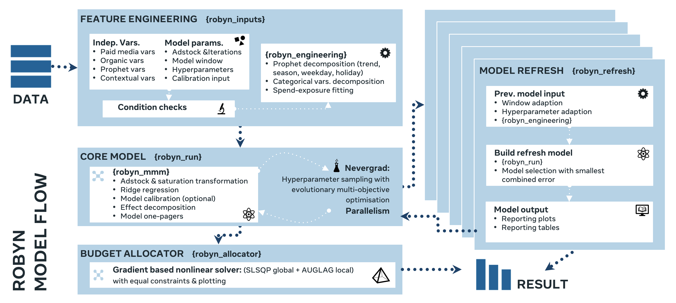
Model flow
Core capabilities
-
Semi-automated modelling process: Robyn automatically returns a set of business-relevant and Pareto-optimum results by optimizing on the model fit and business fit over larger iterations. Building MMM manually is a very time-consuming process that involves many subjective decisions, modelling experience and trial and error over hundreds of iterations. Months of effort is common to build MMM from scratch. Robyn is able to automate a large portion of the modelling process (see Resident case above) and thus reduce the "analyst-bias". Pure model run time for recommended 10k iterations on a laptop is <1 hour. Technically speaking, Robyn leverages the multi-objective optimization capacity of Facebook's evolutionary optimization platform Nevergrad to minimize both prediction error (NRMSE, normalized root-mean-square error) and decomposition distance (DECOMP.RSSD, decomposition root-sum-square distance, a major innovation of Robyn) at the same time and eliminates the majority of "bad models" (larger prediction error and/or unrealistic media effect like the smallest channel getting the most effect).
-
Continuous reporting: After the initial model is built and selected, the new
robyn_refresh()function is able to continuously build model refresh at any given cadence based on previous model result. This capability enables using MMM as a continuous reporting tool and therefore makes MMM more actionable. -
Trend & season decomposition: Robyn leverages Facebook's time-serie-forecast package Prophet to decompose trend, season, holiday and weekday as model predictor out of the box. This capability often increases model fit and reduces autoregressive pattern in residuals.
-
Rolling window: In Robyn 3.0, user can specify
window_startandwindow_endin therobyn_inputs()function to set modelling period to a subset of available data. A, important capability to keep MMM returning up-to-date results frequently. At the same time, baseline variables like trend, season, holiday and weekday are still derived from the entire dataset, ensuring higher accuracy for time-serie decomposition. For example, with Robyn's integrated dataset of 208 weeks, user can set 100 weeks as modelling window while trend, season, holiday and weekday are derived from all 208 weeks. -
Granular dataset: Robyn is able to deal with larger dataset with multicollinearity. It's common to have similar spending pattern among Marketing channels, for example increasing spend for multiple channels around Christmas. Robyn uses Ridge regression to deal with the inherent multicollinearity in Marketing dataset naturally, selects predictors by penalisation natually and prevents overfitting without doing computationally intensive time-serie cross validation.
-
Organic media: In Robyn 3.0, user can specify
organic_varsto model Marketing activities that have no spend. Typically, this includes newsletter, push notification, social media posts etc. Technically speaking, organic variables are expected to have similar carried-over (adstock) and saturating behavior as paid media variables. The respective transformation techniques (Geometric or Weibull transformation for adstock; Hill transformation for saturation) as treatment for these behaviours are now also applied for organic variables. -
Experimental calibration: We believe integrating experimental results into MMM is the best choice for model selection. As the general aphorism in statistics "all models are wrong but some are useful", there's no reliable way to select final MMM results, even after Robyn has accounted for the business fit with the DECOMP.RSSD as objective function. Experiments (RCT, randomised controlled trials) are causal by nature and thus are seen as ground-truth. Common experimental tools include people-based technique like Facebook Conversion Lift and geo-based technique like Facebook GeoLift, among others. Technically speaking, Robyn drives model results closer to experimental results by using MAPE.LIFT as the third objective function besides NRMSE & DECOMP.RSSD when calibrating and minimizing the error between predicted and experimental results.
-
Custom adstock: Robyn offers the one-parametric Geometric function, the two-parametric Weibull CDF (Cumulative Distribution Function) and the two-parametric Weibull PDF (Probability Density Function) as adstock options to enable more customisation and flexibility in adstock transformation. The Geometric adstock is considered more intuitive and runs faster. Weibull CDF adstock is not only more flexible, but often more suitable for digital media transformation, as shown in this study or one attached by Ekimetrics from Ekimetrics. Weibull PDF adstock is the most flexible among all three and enables additional lagged effect.
-
S-shape saturation: Robyn uses the two-parametric Hill function that is able to transform between C- and S-shape to enable more customisation and flexibility in saturation transformation.
-
Budget allocator: Based on selected model result, or to be precise the saturation curve of each paid media variable, the
robyn_allocator()function returns the optimal mix of spend that maximizes the total response. Technically speaking, Robyn uses by default a combination of Augmented Lagrangian (AUGLAG) as global optimization algorithm and Sequential Least Square Quadratic Programming (SLSQP) as local optimization algorithm to solve the nonlinear objective function analytically. -
Automated output: When using
robyn_run()function to build the initial model, Robyn outputs a one-pager that contains 6 charts for every Pareto-optimum model and saves 4 csv-files (pareto_hyperparameters.csv, pareto_aggregated.csv, pareto_media_transform_matrix.csv, pareto_alldecomp_matrix.csv) that contains all results. The 6 charts are: the effect decomposition waterfall chart, the actual vs. predicted fit line chart, the media spend vs. effect bar chart, the media saturation line chart, the adstock decay rate bar chart and the predicted vs. residual line chart. When usingrobyn_refresh()function to build refresh models, Robyn outputs 2 extra charts (aggregated actual vs. predicted line chart and aggregated decomposition bar chart) and saves 4 extra csv-files separately (report_hyperparameters.csv, report_aggregated.csv, report_media_transform_matrix.csv, report_alldecomp_matrix.csv).
Example plots
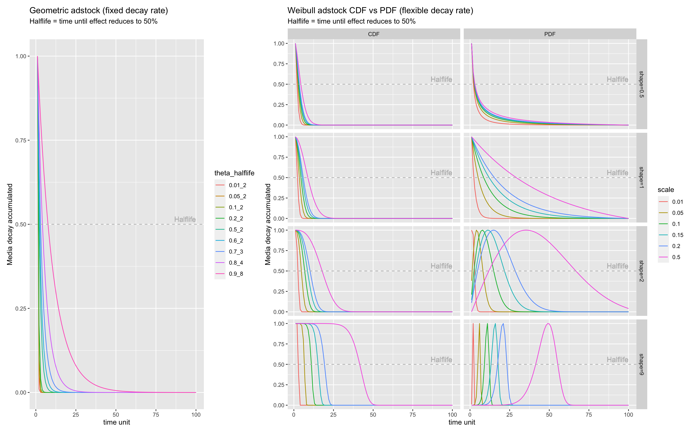
Adstock helper plot
This plot shows how the three adstock options, Geometric, Weibull CDF & Weibull PDF, are transforming as the parameter changes.
-
Geometric adstock: Theta is the only parameter and means fixed decay rate. Assuming TV spend on day 1 is 100€ and theta = 0.7, then day 2 has 100x0.7=70€ worth of effect carried-over from day 1, day 3 has 70x0.7=49€ from day 2 etc. Rule-of-thumb for common media genre: TV c(0.3, 0.8), OOH/Print/Radio c(0.1, 0.4), digital c(0, 0.3)
-
Weibull CDF adstock: The Cumulative Distribution Function of Weibull has two parameters, shape & scale, and has flexible decay rate, compared to Geometric adstock with fixed decay rate. The shape parameter controls the shape of the decay curve. Recommended bound is c(0.0001, 2). The larger the shape, the more S-shape. The smaller, the more L-shape. Scale controls the inflexion point of the decay curve. We recommend very conservative bounce of c(0, 0.1), because scale increases the adstock half-life greatly.
-
Weibull PDF adstock: The Probability Density Function of the Weibull also has two parameters, shape & scale, and also has flexible decay rate as Weibull CDF. The difference is that Weibull PDF offers lagged effect. When shape > 2, the curve peaks after x = 0 and has NULL slope at x = 0, enabling lagged effect and sharper increase and decrease of adstock, while the scale parameter indicates the limit of the relative position of the peak at x axis; when 1 < shape < 2, the curve peaks after x = 0 and has infinite positive slope at x = 0, enabling lagged effect and slower increase and decrease of adstock, while scale has the same effect as above; when shape = 1, the curve peaks at x = 0 and reduces to exponential decay, while scale controls the inflexion point; when 0 < shape < 1, the curve peaks at x = 0 and has increasing decay, while scale controls the inflexion point. When all possible shapes are relevant, we recommend c(0.0001, 10) as bounds for shape; when only strong lagged effect is of interest, we recommend c(2.0001, 10) as bound for shape. In all cases, we recommend conservative bound of c(0, 0.1) for scale. Due to the great flexibility of Weibull PDF, meaning more freedom in hyperparameter spaces for Nevergrad to explore, it also requires larger iterations to converge.
Saturation helper plot
This plot shows how the Hill function transforms as the parameter changes. Hill function is a two-parametric function in Robyn with alpha and gamma. Alpha controls the shape of the curve between exponential and s-shape. Recommended bound is c(0.5, 3). The larger the alpha, the more S-shape. The smaller, the more C-shape. Gamma controls the inflexion point. Recommended bounce is c(0.3, 1). The larger the gamma, the later the inflection point in the response curve.

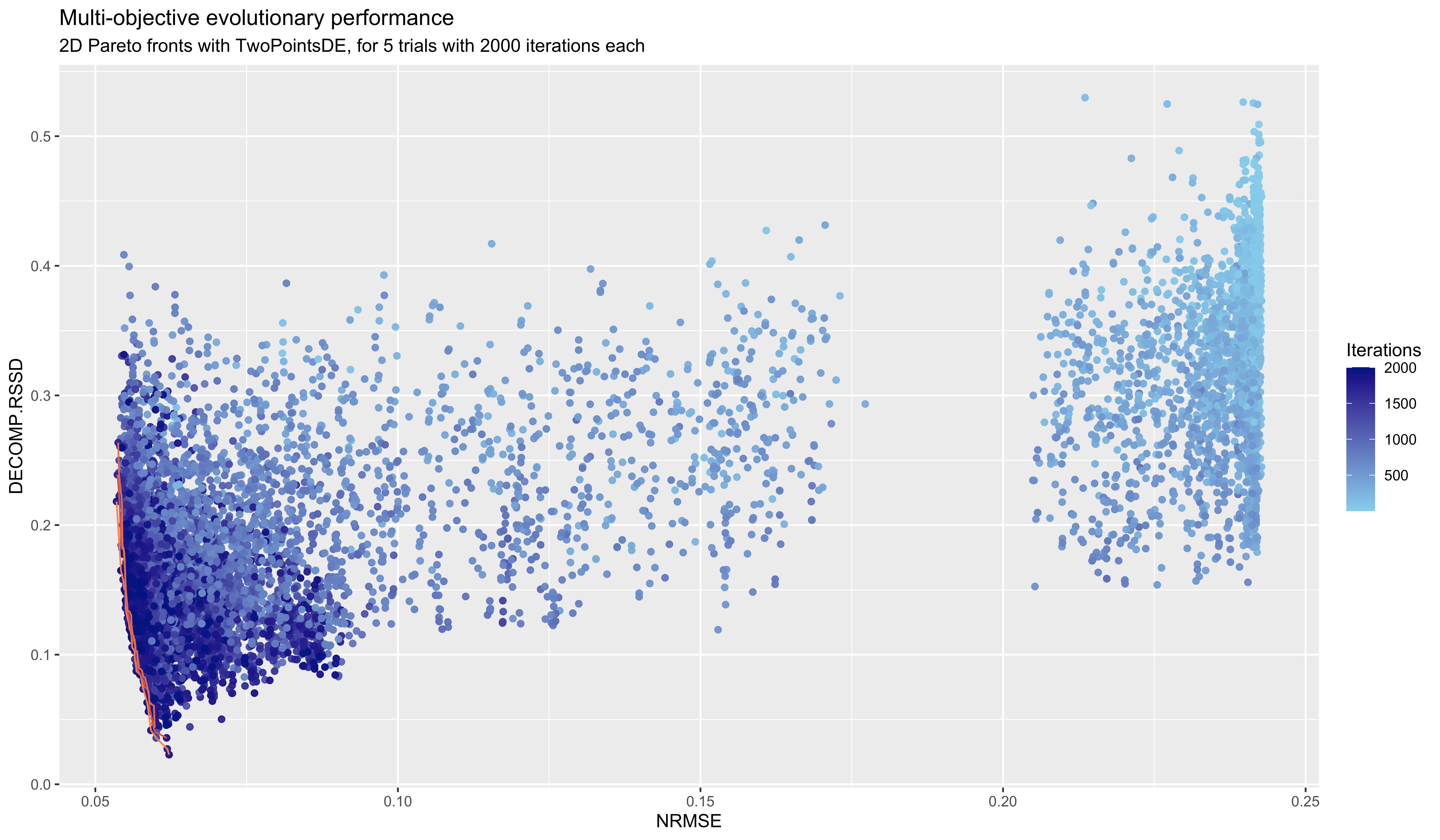
Pareto-front chart for the initial model build
The chart below shows the performance of the multi-objective optimisation from the evolutionary algorithm platform Nevergrad over 10k iterations in total. The two axis (NRMSE on x and DECOMP.RSSD on y) are the two objective functions to be minimised. As the iteration increases, a trend down the lower left corner of the coordinate can be clearly observed. This is a proof of Nevergrad's ability to drive the model result toward desired direction. The red lines are Pareto-fronts 1-3 and contains the best possible model results from all iterations.
Convergence plot per iteration quantile
The convergence of each objective function over iteration is showed. It's clear to observe that the median of both objective functions are trending smaller as iteration increases, while the spread / standard deviation are also getting smaller. There're two rules for convergence. For median, it's considered converged when median of last iteration quantile < mean median of first quantile - 3 * sd from first 3 quantiles. For sd, it's considered converged when sd of last quantile < mean sd of the first 3 quantiles.

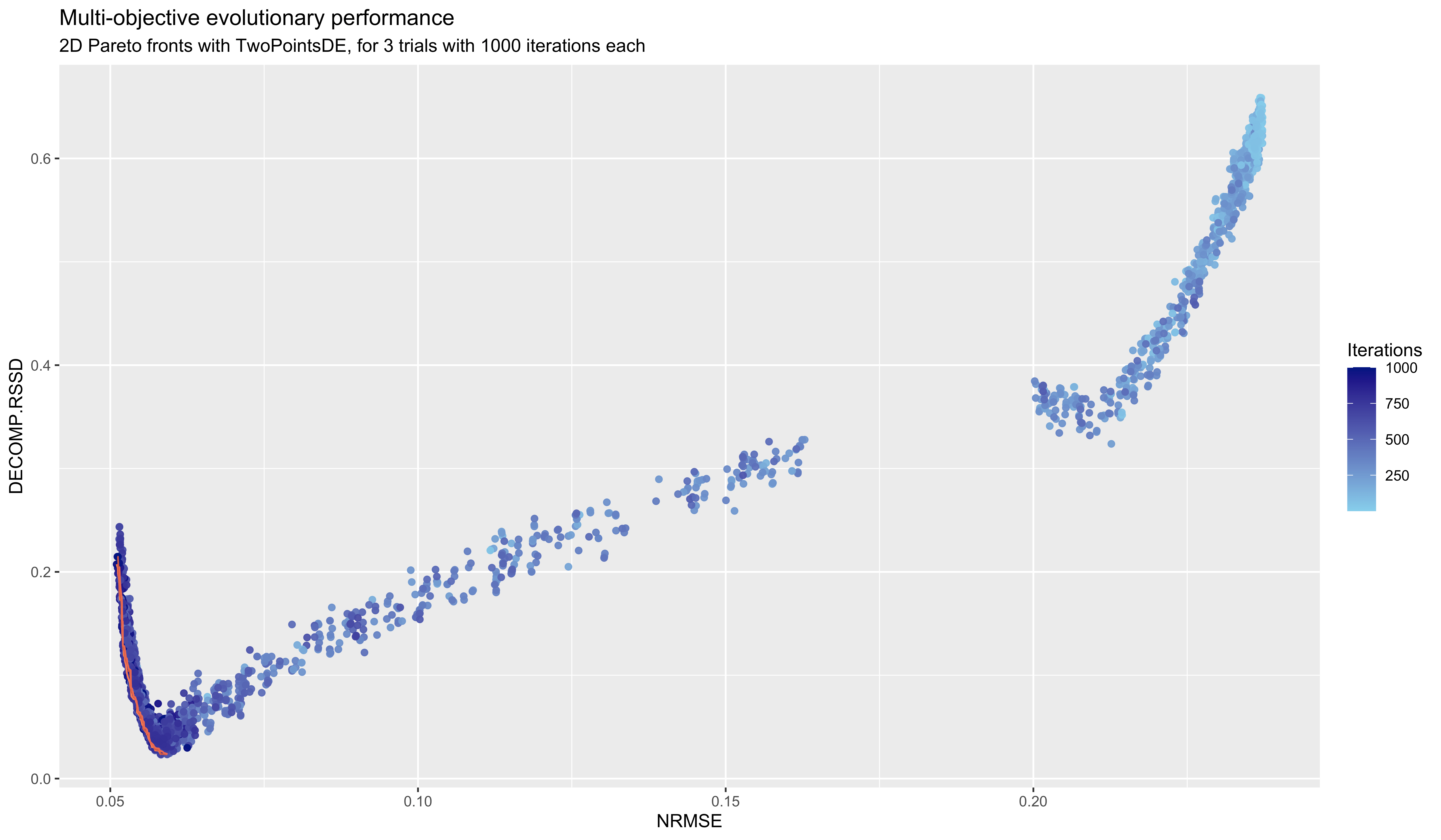
Pareto-front chart for the refresh model build
Similar to initial model above, a more obvious trend of the multi-objective minimization process can be observed during the refreshing process with 3k iterations. The reason for this behaviour is that hyperparameter bounds are narrower during refresh than in the initial build which leads to faster convergence.
ROAS convergence over iterations
The ROAS convergence plot shows how the ROAS for paid media evolves over time and iterations. We know that Nevergrad optimises all objective functions as the iteration grows, and the pareto fronts lie in the later iterations. This behaviour can also be observed from the ROAS point of view. For some channels, it's clear that the higher iterations are producing more "peaky" ROAS distribution, indicating higher confidence for certain channel results. Although, we still believe that the peak doesn't mean the "truth". Experimental calibration remains the single source of truth.

Reporting model refresh time-series fit
All initial and refresh builds are included sequentially. For the refresh builds, only the added new periods will be appended. The assembled R-squared is adjusted and describes the fit of the assembled actual & fitted lines below. Refresh builds can have different window lengths (parameter refresh_step in the robyn_refresh() function).
Reporting model refresh decompsition & ROAS
Decomposition of all predictors per build. The baseline variable is the sum of all prophet variables (trend, season, weekday, holiday) and the intercept. It's often more intuitive to look at baseline variable due to the possible intercept drop in the Ridge regression and the effect shift between these baseline variables. All data is simulated and don't have real-life implication.
Prophet decomposition
Trend, season, holiday and extra regressor ("event" in this case) decomposition by Prophet. Weekday is not used because the sample data is weekly. Robyn uses Prophet to also decompose categorical variables as extra regressor to simplify later programming. For technical details of decomposition, please refer to Prophet's documentation here.
Spend exposure plot
When using exposure variables (impressions, clicks, GRPs etc) instead of spend in paid_media_vars, Robyn fits an nonlinear model with Michaelis Menten function between exposure and spend to establish the spend-exposure relationship. The example data shows very good fit between exposure and spend. However, when a channel has more complex activities, for example a large advertiser having multiple teams using different strategies (bidding, objective, audience etc.) for Facebook ads, it's possible that the high-level channel total impressions and spends will fit poorly. A sign to consider splitting this channel into meaningful subchannels.
Model one-pager
An example of the model one-pager for each Pareto-optimal models. All data is simulated and don't have real-life implication.
- Waterfall chart: Total decomposition of all independent variables
- Predicted vs. actual chart: Visual examination of the time-serie fit of the model prediction
- Media decomposition chart: Media share of spend vs share of effect with ROAS (CPA when using conversions as dependent variable). This also shows the intuition of the objective function DECOMP.RSSD decomposition distance.
- Saturation curves: The Hill function induced saturation curves for each media variable.
- Average media decay rate: Decay rate comparison. When using Geometric adstock, this equals to theta. When using Weibull, because Weibull is two-parametric with changing decay rate over time that is difficult to illustrate intuitively, we've chosen to compare the total Weibull infinite sum of decay to it's equivalent in Geometric's infinite sum of decay rate and finally plot the Geometric decay rate as a visual approximate to the Weibull average decay.
- Fitted vs. residuals: Visual examination of the model diagnostic in residuals
Budget allocator
For every selected model result, the robyn_allocator() function can be applied to get the optimal budget mix that maximizes the response. It has two scenarios:
- Maximum historical response: It simulates the scenario "how much lift in response can be achieved with which budget mix given the same average spend level in history?"
- Maximum response for expected spend: It simulates the scenario "how much lift in response can be achieved given a specific spend level for a given period?" Robyn's budget allocator uses the gradient-based nloptr library to solve the nonlinear saturation function (Hill) analytically. For more details please check the vignette of the nloptr library.
Q&A
Input data questions
-
What is the rationale behind using exposure metrics (impressions, clicks, GRPs etc.) instead of spend to represent paid media in
paid_media_vars: See here and here. -
How many data points/how long time period should I include in the model?: See here.
Core modelling questions
-
How is decomposition distance DECOMP.RSSD calculated? What's the rationale behind?: See here.
-
Can DECOMP.RSSD limit the model's ability to detect over- or underperforming channels?: See here.
-
How are adstock and saturation transformation applied in Robyn?: See here.
-
How does Robyn's budget allocator work?: See here.
-
Does Robyn do time-serie cross-validation to prevent overfitting?: See here.
Output interpretation questions
-
What are the best practices to select final model among all Pareto-optimum output?: See here.
-
Does Robyn return uncertainty metrics like p-value or confidence interval for predictors?: See here.
-
Robyn returns either zero or too high effect & ROI for certain media variables. Is it possible to force it?: See here.
-
Can Robyn account for interative/synergy effect between channels?: here.
Nevergrad algorithm selection
We've conducted a high-level comparison of Nevergrad algorithms aiming to identify the best option for Robyn. At first, we ran 500 iterations and 10 trials for all options. X axis is accumulated seconds and Y axis is combined loss function sqrt(sum(RMSE^2,DECOMP.RSSD^2)). The lower the combined error, the better the model. We can observe that DE (Differential Evolution) and TwoPointsDE are not only achieving the lowest error. They also show the ability to improve continuously, as opposed to OnePlusOne or cGA, for example, that are reaching convergence early and stop evolving.
As deepdive for both differential algorithms, we've ran 2000 iterations for 5 trials as our common recommendation. Y axis is the combined error and X axis the iteration counts. We can observe that both algorithms are reaching the "flat tail" after 1000 iterations, although small improvements are still happening. Both algorithm are having similar level of combined error. Based on this, we selected "TwoPointsDE" as the standard Nevergrad algorithm.
Release log
-
Robyn 3.0.0 release (2021-09-29)
-
Robyn 2.0.0 release (2021-03-03)
-
Robyn 1.0.0 release (2020-11-30)
License
FB Robyn MMM R script is MIT licensed, as found in the LICENSE file.
- Terms of Use - https://opensource.facebook.com/legal/terms
- Privacy Policy - https://opensource.facebook.com/legal/privacy
- Defensive Publication - https://www.tdcommons.org/dpubs_series/4627/
Contact
- [email protected], Gufeng Zhou, Marketing Science Partner
- [email protected], Leonel Sentana, Marketing Science Partner
- [email protected], Igor Skokan, Marketing Science Partner
- [email protected], Bernardo Lares, Marketing Science Partner