
Super-Sunshine
A ray-tracer with a simple scene description language for easily generating beautiful images.

Summary
Super-Sunshine is a ray-tracer that can be easily interacted with. The diagram below illustrates the manner in which this interaction is meant to occur:

As an example, let's say you wanted to render an image of three scoops of ice cream sitting in the middle of a desert. Using the scene description language developed for this project, you would start by writing a scene description like the following:
# Setup
size 640 480
output ice_cream.png

# Camera
camera 1.5 3.5 1.5 -0.5 0 -0.5 0 1 0 45

# Point light
attenuation 0 1 0
point 0.4 3.75 -1.6 1 1 1

# Common material
diffuse 0 0.75 0
shininess 100

# Scoops of ice cream (3 spheres)
ambient 0.122 0.541 0.439
sphere -0.6 0.375 -0.6 0.375
ambient 0.745 0.859 0.224
sphere -0.6 1.05 -0.6 0.3
ambient 0.9 0.9 0.102
sphere -0.6 1.575 -0.6 0.225

# Reflective material
specular 0 0.25 0

# Vertices
maxverts 4
vertex 0.7125 0 0.7125
vertex 0.7125 0 -1.9125
vertex -1.9125 0 0.7125
vertex -1.9125 0 -1.9125

# Desert floor (2 triangles)
ambient 0.992 0.455 0
tri 0 1 2
tri 1 3 2
You would then give your scene description to Super-Sunshine, which would read it and turn it into an image like the one below:

Dessert on a desert!
As you can see, the scene description language makes it easy to play with the ray-tracer. As an additional benefit, it also enables you to generate animations through scripting; it is hard to believe how such a simple feature can lead to such stunning results:

A very narcissistic flower.
Technical details
This project started out as a final assignment for Ravi Ramamoorthi's fantastic course on computer graphics. Since then, it has continued to grow because it provides a great environment for experimenting with new computer graphics concepts. In its current form, the project consists of:
- A recursive ray-tracer.
- A file parser designed to read scene descriptions written with a simple scene description language.
- A linear algebra API for performing operations with points, vectors, normals and affine transformation matrices.
All the code was written in C++, with a strong focus on making it clear and organized. The only external library used is the FreeImage library (it is used to generate PNG images with the RGB values calculated by the ray-tracer).
To compile the project in macOS or Linux, simply use the Makefile included in this repository (thanks to Yarden Arane and Daniel Macario for helping with the cross-platform support!).
Features
The scene description language developed for this project is very simple. In terms of syntax, you only need to know two things:
- Comments start with a number sign:
# This is a comment.- Commands consist of a keyword followed by a series of parameters, each separated by at least one space:
keyword parameter1 parameter2 ...Below you will find information on all the commands that are currently supported. They are separated into seven different categories: Setup, Camera, Geometry, Transformations, Lights, Materials and Textures.
Note that once you are done writing a scene description, you can give it to the ray-tracer by specifying its filename as a command-line parameter:
$ super_sunshine scene.txt1) Setup
In a scene description, there are three parameters that must be specified before any others. The first two are the dimensions of the image that will be generated by the ray-tracer, and the third one is the filename of said image. The commands used to set these parameters are the following:
size width height
output filename.png
Where:
- width and height are the desired dimensions in pixels.
- filename is the filename that will be assigned to the PNG image.
2) Camera
A camera must be specified to define how a scene is framed. This is done with the following command:
camera fromx fromy fromz atx aty atz upx upy upz fovyWhere:
- from is the point at which the camera is located.
- at is the point that the camera points to.
- up is the vector that defines which way is up for the camera.
- fovy is the field of view in the Y direction.
In the animation below, the from point is rotated along a 45° arc while the at point remains fixed at the center of the pyramid's base.

A lonely pyramid.
3) Geometry
Two geometric primitives are currently supported: spheres and triangles. Two doesn't sound like much, but remember you can make any shape with just triangles:

This rendering of the Stanford Dragon is made out of 100 thousand triangles (scene description from CSE167x).
A sphere is created using this command:
sphere centerx centery centerz radiusWhere:
- center is the point at which the sphere is centered.
- radius is the radius of the sphere.
In the case of a triangle, it is created as follows:
maxverts max
vertex posx posy posz
vertex posx posy posz
vertex posx posy posz
tri index1 index2 index3
Where:
- maxverts is the command used to define the maximum number of vertices (max) that can be created in a scene description. This value is used by Super-Sunshine to allocate the size of a few data structures, so it must be specified before creating any vertices. Since it is an upper limit, it does not have to match the exact number of vertices that are actually created.
- vertex is the command used to create a single vertex at point pos.
- tri is the command used to create a triangle. Its three parameters are the indices of three vertices. The first vertex you create with the vertex command has index zero, and this value increases by one for each subsequent vertex you create. Note that the indices must be specified in a counterclockwise order so that the normal of the triangle points in the correct direction. Also keep in mind that different triangles can share vertices (e.g. you should be able to make a square by only creating 4 vertices and 2 triangles).
4) Transformations
Three basic transformations are currently supported: translations, rotations and scaling. The commands for these transformations are:
translate x y z
rotate x y z angle
scale x y z
Where:
- translate translates a geometric primitive x, y and z units along the X, Y and Z axes, respectively.
- rotate rotates a geometric primitive counterclockwise by angle degrees about the vector defined by x, y and z.
- scale scales a geometric primitive by x, y and z units along the X, Y and Z axes, respectively.
The image below illustrates a simple use case of these transformations:

The planet Tralfamadore.
You might be surprised to learn that...
- The rings are made out of spheres that were squashed along the Y axis using the scale command.
- The slight tilt of the rings was achieved by rotating them about the X and Z axes using the rotate command.
- The stars are copies of the planet that were moved very far away using the translate command.
Just as in OpenGL, these transformations right multiply the model-view matrix. This means that the last transformation specified is the first one to be applied. For example, if you wanted to:
- Create a sphere of radius 1.5 centered at the origin.
- Scale it by a factor of 2.
- Rotate it clockwise by 90° about the Y axis.
- Translate it -5 units along the Z axis.
You would write the following:
translate 0 0 -5
rotate 0 1 0 -90
scale 2 2 2
sphere 0 0 0 1.5
The order of the commands might seem odd at first, but if you read them from the bottom to the top they match the verbal description of what we wanted to achieve. So if you are ever confused about the order in which transformations apply to a specific geometric primitive, you can always rely on this rule of thumb: read from the command that creates the geometric primitive to the beginning of the scene description, and apply transformations as you run into them. Also keep in mind that the order in which transformations are specified does matter: rotating and then translating is not the same as translating and then rotating.
Additionally, the commands pushTransform and popTransform are also supported. These two commands imitate the syntax and functionality of their counterparts in old-school OpenGL, allowing you to apply transformations to specific geometric primitives without affecting others. To better understand their use and the order in which transformations are applied, consider the following example:
translate 1 0 0

pushTransform
   rotate 0 1 0 45
   sphere 0 0 0 1
popTransform

sphere 0 1 0 0.5- The sphere that is inside the push/pop block is centered at (0, 0, 0) and has a radius of 1. The first transformation applied to it is the nearest one moving towards the top. In this case it is a 45° counterclockwise rotation about the Y axis. The next transformation is a translation of 1 unit along the X axis.
- The sphere that is outside the push/pop block is centered at (0, 1, 0) and has a radius of 0.5. Since it is not inside the push/pop block, the 45° counterclockwise rotation about the Y axis does not apply to it. Its first transformation then ends up being the translation of 1 unit along the X axis.
Transformations can be intimidating at first, but play around with them for a while and they will start to make sense!
5) Lights

Salesman: Have you thought much about luggage, Mr. Banks?
Mr. Banks: No, I never really have.
Salesman: It is the central preoccupation of my life.
Replace the word luggage with the word light, and you could say that I am the salesman in that scene. My obsession with light is so bad, in fact, that I had to rewrite this section about a dozen times, because I kept going off track talking about Maxwell’s equations. Thankfully, we do not have to worry about those equations, because a ray-tracer's approach to modeling light is very simple.
What we do have to worry about are the different types of light sources that we can have in a scene. As an experiment, look around you and take note of all the light sources that you see. Perhaps you are sitting next to a window, and sunlight is pouring in through it. Maybe there is a lamp close by with a warm light bulb. Or a few shiny surfaces that reflect the light emitted by other sources. These are all light sources with different behaviours, which is why each one is modeled differently.
The three subsections below will teach you how to create light sources like the ones I mentioned above, and they will give you some background on how they are modeled.
5.1) Ambient light
Ambient light is the simplest light source available. Once included in a scene, it illuminates all geometric primitives with equal intensity, regardless of their positions or orientations in space. By doing this, it models the uniform illumination produced by rays of light that have been reflected many times.
The command used to set the colour of this light source is:
ambient r g bWhere the RGB values can range from 0 to 1.
Once the colour is set, it applies to all the geometric primitives created afterwards. Unless, of course, you change it by using the ambient command again, in which case the new colour begins to apply. As an example of this, consider the following snippet, in which I create four spheres under four different ambient light colours:
# Left sphere (green)
ambient 0.2 0.4 0.1
sphere -0.75 0 -2 0.5

# Right sphere (yellow)
ambient 0.7 0.7 0
sphere 0.75 0 -2 0.5

# Bottom sphere (red)
ambient 0.75 0 0
sphere 0 -0.75 -2 0.5

# Top sphere (blue)
ambient 0 0.262 0.344
sphere 0 0.75 -2 0.5
The resulting image looks like this:

One ambient light shining four different colours.
This behaviour is very particular, but it is convenient in the context of a ray-tracer. Just remember that when you create a geometric primitive, it stores the current colour of the ambient light, just as it stores the current transformations and material properties. Also note that if you do not specify the colour of the ambient light, it defaults to (0.2, 0.2, 0.2).
5.2) Point lights
A point light is a light source with two defining characteristics:
- It emits light in all directions from a specific point in space.
- The intensity of the light it emits decreases with the distance from its origin.
The second bullet point describes what is known as distance falloff or attenuation, which is a phenomenon whose consequences you see every day: objects that are close to a light source are illuminated brightly, while those that are far away are not.
In nature, the intensity of light decreases quadratically, that is, with the square of the distance from its origin. In Super-Sunshine, you can choose to have the intensity not decrease at all, or to have it decrease in a constant, linear or quadratic manner.
The commands used to create a point light with a specific form of attenuation are:
attenuation constant linear quadratic
point posx posy posz r g b
Where:
- attenuation is the command used to define the way in which light is attenuated. By default, there is no attenuation, which means that the attenuation coefficients are equal to (1, 0, 0).
- point is the command used to create a point light at point pos. The colour of the emitted light is determined by the RGB values.
If you wanted the intensity of the light emitted by a point light to decrease linearly with the distance from its origin, you would set the attenuation coefficients to (0, 1, 0). If you wanted it to decrease quadratically, you would use (0, 0, 1). Note that you can also combine the different forms of attenuation and use coefficients larger than 1 to make the intensity decrease even faster. Also note that you can create multiple point lights with different attenuations by changing the attenuation before creating each one.
The animation below contains two quadratically-attenuated point lights (one at the upper-left corner and the other at the lower-right corner):

A green rupee from Ocarina of Time!
5.3) Directional lights
A directional light is commonly viewed as an unattenuated point light that has been placed infinitely far away. Because this point light is so far away, the rays of light it emits arrive parallel to each other at any given scene. This means that a directional light has one defining characteristic: it only emits light in a single direction.
The command used to create a directional light is:
directional dirx diry dirz r g bWhere:
- dir is the vector that defines the direction in which light is emitted, while the RGB values determine the colour of the light.
Before moving on to the material properties, consider this question: what type of light source would you use to model sunlight?
When I was first asked that question, my answer was: "Well ambient light of course! When you are outside, the sun illuminates everything around you uniformly". This seemed natural to me, but let's think about it carefully:
- The sun is 149.6 million kilometers away from earth. Because this distance is so large, we can think of the sun as a point light that has been placed infinitely far away (at least until humanity figures out how to travel at the speed of light, in which case no distance will be too large).
- The position of the sun affects the way it illuminates objects. Things do not look the same at dawn and at noon, do they?
Now it seems a lot more natural to use a directional light!
6) Materials
Super-Sunshine uses the Blinn-Phong shading model to compute the colours of the geometric primitives in a scene. In this section, I will illustrate how this model works by detailing the steps it follows to render a simple scene: a single sphere illuminated by a single point light. The diagram below depicts how the scene is arranged:

We will assume that the point light emits white light, which means that its colour is (1, 1, 1), and that it is not affected by any form of attenuation. As for the material properties, I will reveal them as we run into them. So let's get to it!
Step 1: Ambient light and emissivity.
The first thing we need to do is check if the sphere has an associated ambient light colour and emissivity. You already know where the ambient light colour comes from and how it behaves, but what about the emissivity? This material property models the intrinsic colour of an object. It behaves exactly like ambient light, and it is set using the following command:
emission r g bWhere the RGB values determine the colour of the emissivity.
Let's say that the sphere in our scene has an ambient light colour of (0, 0, 0.125) and an equal emissivity. These two values added together form the base colour of the entire sphere. Since colour addition is performed component-wise, the result is (0, 0, 0.25), which corresponds to a dark shade of blue.
The image below illustrates what the sphere looks like under the conditions we have specified so far:

Ambient light + Emissivity
Things look a little flat, don't they?
Step 2: Diffuse reflections.
The next thing we need to do is create the illusion of depth. To achieve this, we need the parts of the sphere that face the point light to be illuminated brightly, the ones that are angled with respect to it to be partially illuminated, and the ones that face away from it to be in shadows.
But how do we generate this colour gradient? This is where the Blinn-Phong shading model is exceedingly clever. It establishes two conditions:
- When a point on the sphere is struck by a ray of light, the colour of the ray is added to the colour of the point.
- The intensity of a ray of light varies depending on the angle at which it strikes the sphere.
To illustrate these concepts, take a look at the diagram below, which depicts three points on the sphere being struck by rays of light:

Let's calculate the colour of each of the three points (ignoring the ambient light and the emissivity):
- Point A: The angle between its normal and the incident ray of light is 0°, which means that it faces the point light directly. Because of this, it should be illuminated with the full intensity of the point light. The colour of this point would then be (1, 1, 1), or white.
- Point B: The angle between its normal and the incident ray of light is 90°, which means that the ray is tangent to it. We consider this to be equivalent to the ray not striking the point, which is why it should not be illuminated at all. The colour of this point would then be (0, 0, 0), or black.
- Point C: The angle between its normal and the incident ray of light is 45°. Because of this, it should be illuminated with half of the intensity of the point light. The colour of this point would then be (0.5, 0.5, 0.5), or grey.
For any other point on the sphere, we simply need to scale the intensity of the point light with the cosine of the angle formed between the normal at the point and the incident ray of light, which is exactly what I did for points A, B and C.
The image below illustrates what the sphere would look like if we performed the calculations described above for every point on its surface (ignoring the ambient light and the emissivity):

Diffuse reflections without a colour filter.
Now that's what I call depth! We can even add an additional degree of freedom through what is called the diffuse reflection coefficient. This material property models the way an object absorbs certain wavelengths and reflects others. We can use it to filter the colours of incident rays of light, so that only specific proportions of their RGB values are considered during the calculations described above. It is set using the following command:
diffuse r g bWhere the RGB values define how incident rays of light are filtered.
Let's say that we wanted the sphere to completely ignore the green component of the rays of light that strike it, and that we wanted it to only consider 50% of their red and blue components. To achieve this, we would set the diffuse reflection coefficient to (0.5, 0, 0.5). Since the colour of the point light is (1, 1, 1), all the rays striking our sphere would then have a colour of (0.5, 0, 0.5), or purple. The image below illustrates what the sphere would look like with this diffuse reflection coefficient (ignoring the ambient light and the emissivity):

Diffuse reflections with a colour filter.
Putting the ambient light, emissivity and diffuse reflection coefficient together, the sphere begins to look very beautiful:

Ambient light + Emissivity + Diffuse reflections
Step 3: Specular reflections.
The last thing we need to do to increase the realism of the scene is to add a specular highlight to the sphere. The calculations involved in determining the position of a specular highlight are elaborate, since they take into account the positions of both the light source that produces the highlight and the camera. For this reason, I have decided not to describe them in detail. Instead, I will limit this section to showing you how to control the colour and the size of a specular highlight.
The colour is controlled through what is called the specular reflection coefficient. Just like the diffuse reflection coefficient, this material property acts like a filter of incident rays of light. It is set using the following command:
specular r g bWhere the RGB values define how incident rays of light are filtered.
As for the size of the specular highlight, it is controlled with the shininess coefficient. This material property determines how shiny an object is. It can be set to any number greater than or equal to 0, and it works like this:
- The smaller the shininess coefficient is, the rougher an object is, and consequently the bigger its specular highlight is.
- The bigger the shininess coefficient is, the shinier an object is, and consequently, the smaller its specular highlight is.
This material property is set using the following command:
shininess coefficient Where the coefficient value determines how shiny an object is.
Let's say that we wanted a specular highlight that was large and dark red. First we would need to set the specular reflection coefficient to (0.5, 0, 0), which would make us ignore the green and blue components of incident rays of light while only using 50% of their red components in our highlight calculations. Then we would need to set the shininess coefficient to a small value like 10. With only these material properties, the sphere would look like this:

A specular highlight by itself.
A bit weird, eh? But if we combine all the material properties we have discussed so far, we get a glimpse at the final appearance of the sphere:

Rough sphere.
Now that's better! I do, however, like shiny objects, so let's increase the shininess coefficient to 100:

Shiny sphere.
As you can see, the Blinn-Phong shading model offers fantastic flexibility. It can even support multiple light sources without effort: it simply computes their contributions separately and adds them together at the end.
You should also know that if a geometric primitive has a nonzero specular reflection coefficient, the rays of light that strike it will be reflected off of its surface. And if those reflected rays strike other geometric primitives, their reflections will be displayed on the surface of the first one. This is illustrated in the image below, which contains four spheres with extremely large reflection coefficients:

Single reflections.
But that's not all! We can allow rays to continue reflecting off of the spheres in the scene, creating a hall of mirrors effect. The number of times we permit rays to be reflected is defined with the command-below:
maxdepth depthWhere the depth value sets the upper limit for the number of times rays can be reflected. By default, it is equal to five.
In the previous image, I set the maximum depth equal to one. In the one below, I left it at the default value of five:

Multiple reflections.
I think the previous image doesn't do this effect justice, so I included a close-up:

One doesn't get to use the word "kaleidoscopic" very often, which is why I am very pleased to say that this image is totally kaleidoscopic.
7) Textures
This section is currently under development (thanks to Yarden Arane for writing the code to support textures and colour interpolation, and for generating the really cool image below!).

A man disappointed by a precarious fireworks display.
Future improvements
There is still so much that remains to be done! The more I read about computer graphics, the more I want to continue exploring this field. I really wish my job involved anything related to graphics, or at least a little linear algebra. For now I will continue reading graphics textbooks on my super long commute. If you ever see a guy programming on a bus or metro in Montreal, it is probably me, and I will probably be working on implementing:
- Anti-aliasing (you can blame the saw-like patterns you see in the images above on the lack of this feature).
- Acceleration structures (I reduced the number of operations performed for each pixel as much as I could, but to truly speed things up I must implement acceleration structures).
- Refractive materials (good old Snell's law is not going to implement itself!).
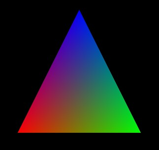
- Surfaces with interpolated normals (this feature will allow users to generate things like RGB triangles).
- Colour bleeding (it would be really cool to generate a Cornell Box).
Learning resources
If you are interested in learning more about computer graphics, I recommend you get started in the following places:
- CSE167x: This EDX course is taught by Ravi Ramamoorthi. It covers the basic linear algebra concepts you need to understand computer graphics, as well as the derivations of many fundamental equations. It uses OpenGL to illustrate the concepts discussed in the lectures, and the final project consists of building a big part of what this readme describes!
- Learn OpenGL: This site is maintained by Joey de Vries. It teaches computer graphics with OpenGL, and it is full of excellent examples and diagrams!
- Scratch a Pixel: This site is similar to the previous one, and it has a section that covers the basics of ray-tracing!
- Real-Time Rendering: This book, written by Tomas Akenine-Möller, Eric Haines and Naty Hoffman, is absolutely invaluable. It compiles hundreds of sources and presents them with brilliant clarity.
I think building a ray-tracer is a really fun project because all the effort you put into it yields actual images that you can marvel at. Just the sheer excitement of generating your first image will keep you motivated while you learn new things! I felt elated when Super-Sunshine spat this out:

The first image generated by Super-Sunshine.
Dedication
This last image is for Venezuela and all of its citizens.
