umapr

umapr wraps the Python implementation of UMAP to make the algorithm accessible from within R. It uses the great reticulate package.

Uniform Manifold Approximation and Projection (UMAP) is a non-linear dimensionality reduction algorithm. It is similar to t-SNE but computationally more efficient. UMAP was created by Leland McInnes and John Healy (github, arxiv).

Recently, two new UMAP R packages have appeared. These new packages provide more features than umapr does and they are more actively developed. These packages are:

• umap, which provides the same Python wrapping function as umapr and also an R implementation, removing the need for the Python version to be installed. It is available on CRAN.

• uwot, which also provides an R implementation, removing the need for the Python version to be installed.

Contributors

Angela Li, Ju Kim, Malisa Smith, Sean Hughes, Ted Laderas

umapr is a project that was first developed at rOpenSci Unconf 2018.

Installation

First, you will need to install Python and the UMAP package. Instruction available here.

Then, you can install the development version from GitHub with:

# install.packages("devtools")
devtools::install_github("ropenscilabs/umapr")

Basic use

Here is an example of running UMAP on the iris data set.

library(umapr)
library(tidyverse)

# select only numeric columns
df <- as.matrix(iris[ , 1:4])

# run UMAP algorithm
embedding <- umap(df)

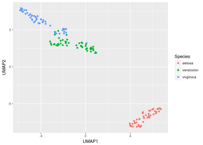
umap returns a data.frame with two attached columns called "UMAP1" and "UMAP2". These columns represent the UMAP embeddings of the data, which are column-bound to the original data frame.

# look at result
head(embedding)
#>   Sepal.Length Sepal.Width Petal.Length Petal.Width    UMAP1     UMAP2
#> 1          5.1         3.5          1.4         0.2 5.647059 -6.666872
#> 2          4.9         3.0          1.4         0.2 4.890193 -8.130815
#> 3          4.7         3.2          1.3         0.2 4.397037 -7.546669
#> 4          4.6         3.1          1.5         0.2 4.412886 -7.633424
#> 5          5.0         3.6          1.4         0.2 5.707233 -6.863213
#> 6          5.4         3.9          1.7         0.4 6.442851 -5.726554

# plot the result
embedding %>% 
  mutate(Species = iris$Species) %>%
  ggplot(aes(UMAP1, UMAP2, color = Species)) + geom_point()

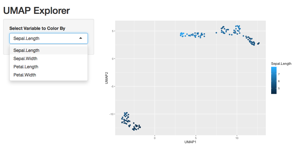
There is a function called run_umap_shiny() which will bring up a Shiny app for exploring different colors of the variables on the umap plots.

run_umap_shiny(embedding)

Function parameters

There are a few important parameters. These are fully described in the UMAP Python documentation.

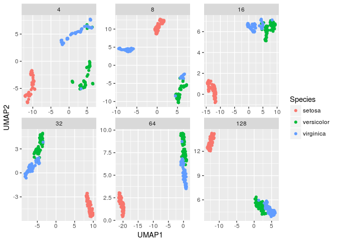
The n_neighbor argument can range from 2 to n-1 where n is the number of rows in the data.

neighbors <- c(4, 8, 16, 32, 64, 128)



neighbors %>% 
  map_df(~umap(as.matrix(iris[,1:4]), n_neighbors = .x) %>% 
      mutate(Species = iris$Species, Neighbor = .x)) %>% 
  mutate(Neighbor = as.integer(Neighbor)) %>% 
  ggplot(aes(UMAP1, UMAP2, color = Species)) + 
    geom_point() + 
    facet_wrap(~ Neighbor, scales = "free")

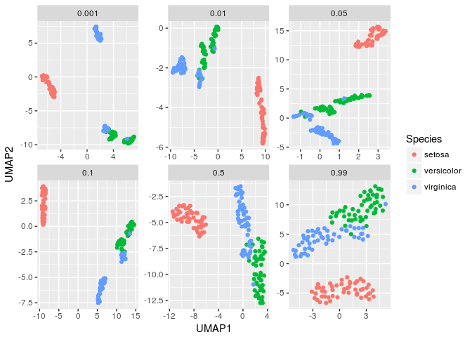
The min_dist argument can range from 0 to 1.

dists <- c(0.001, 0.01, 0.05, 0.1, 0.5, 0.99)

dists %>% 
  map_df(~umap(as.matrix(iris[,1:4]), min_dist = .x) %>% 
      mutate(Species = iris$Species, Distance = .x)) %>% 
  ggplot(aes(UMAP1, UMAP2, color = Species)) + 
    geom_point() + 
    facet_wrap(~ Distance, scales = "free")

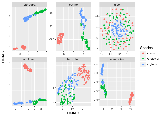
The distance argument can be many different distance functions.

dists <- c("euclidean", "manhattan", "canberra", "cosine", "hamming", "dice")

dists %>% 
  map_df(~umap(as.matrix(iris[,1:4]), metric = .x) %>% 
      mutate(Species = iris$Species, Metric = .x)) %>% 
  ggplot(aes(UMAP1, UMAP2, color = Species)) + 
    geom_point() + 
    facet_wrap(~ Metric, scales = "free")

Comparison to t-SNE and principal components analysis

t-SNE and UMAP are both non-linear dimensionality reduction methods, in contrast to PCA. Because t-SNE is relatively slow, PCA is sometimes run first to reduce the dimensions of the data.

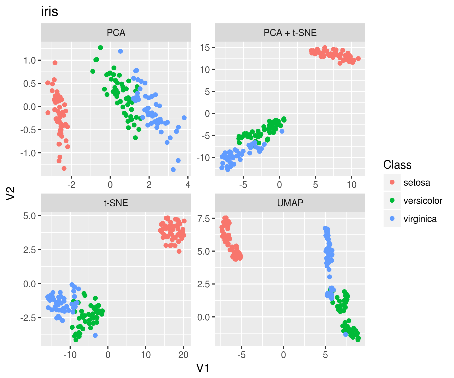
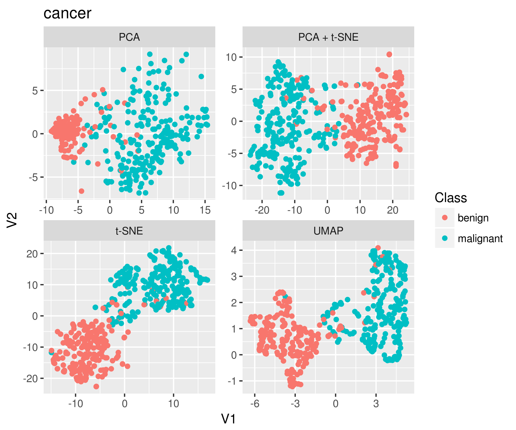
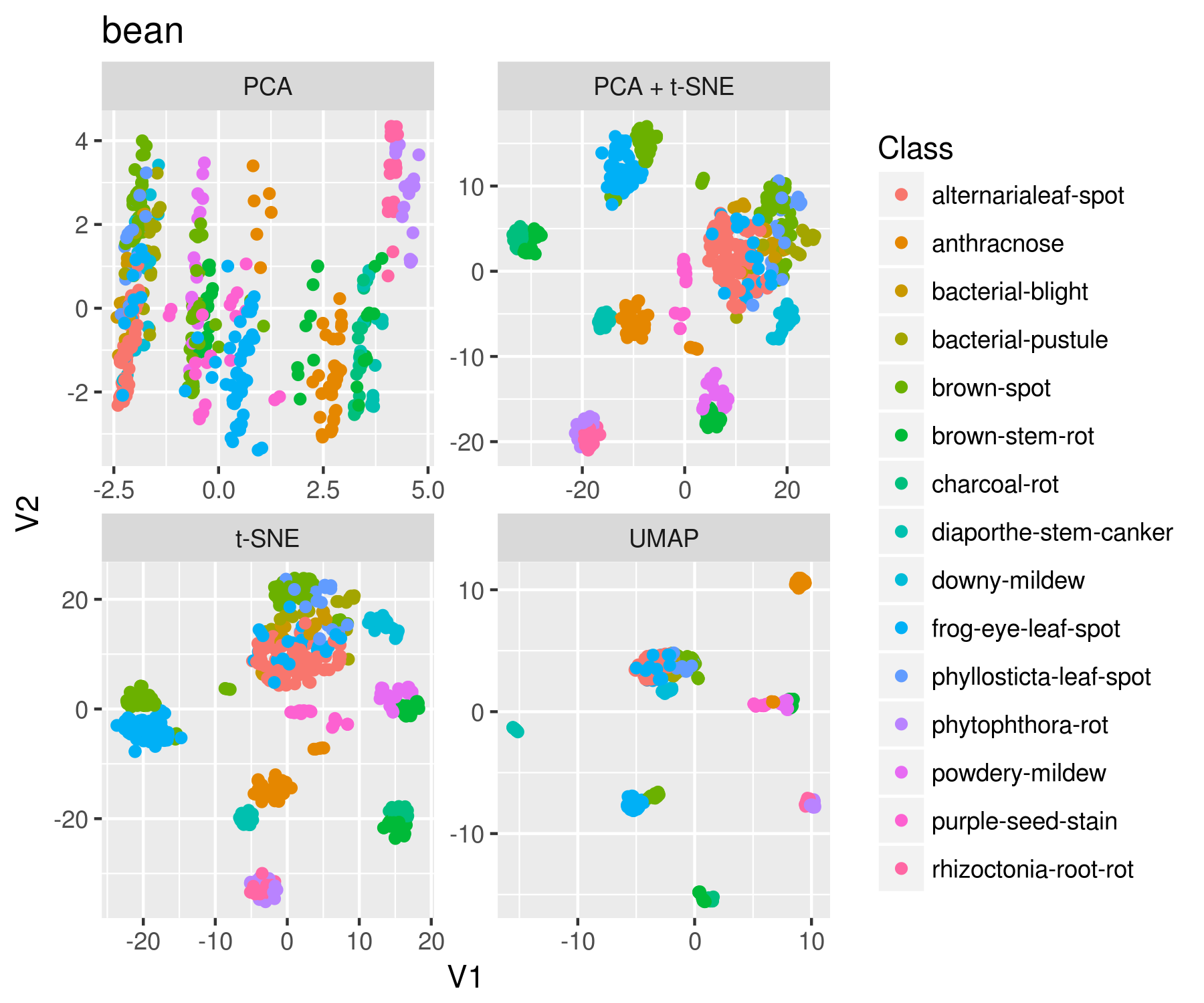
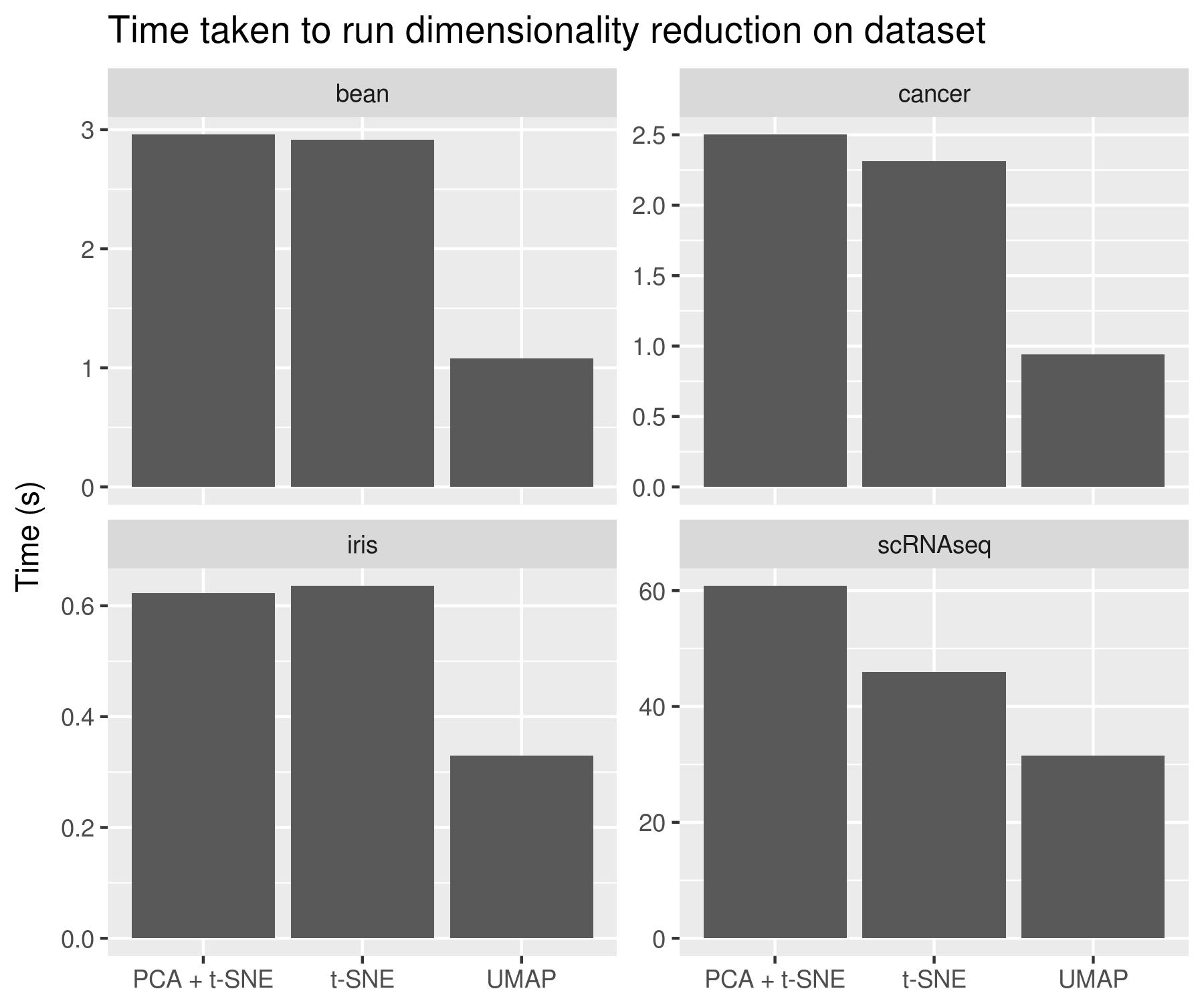
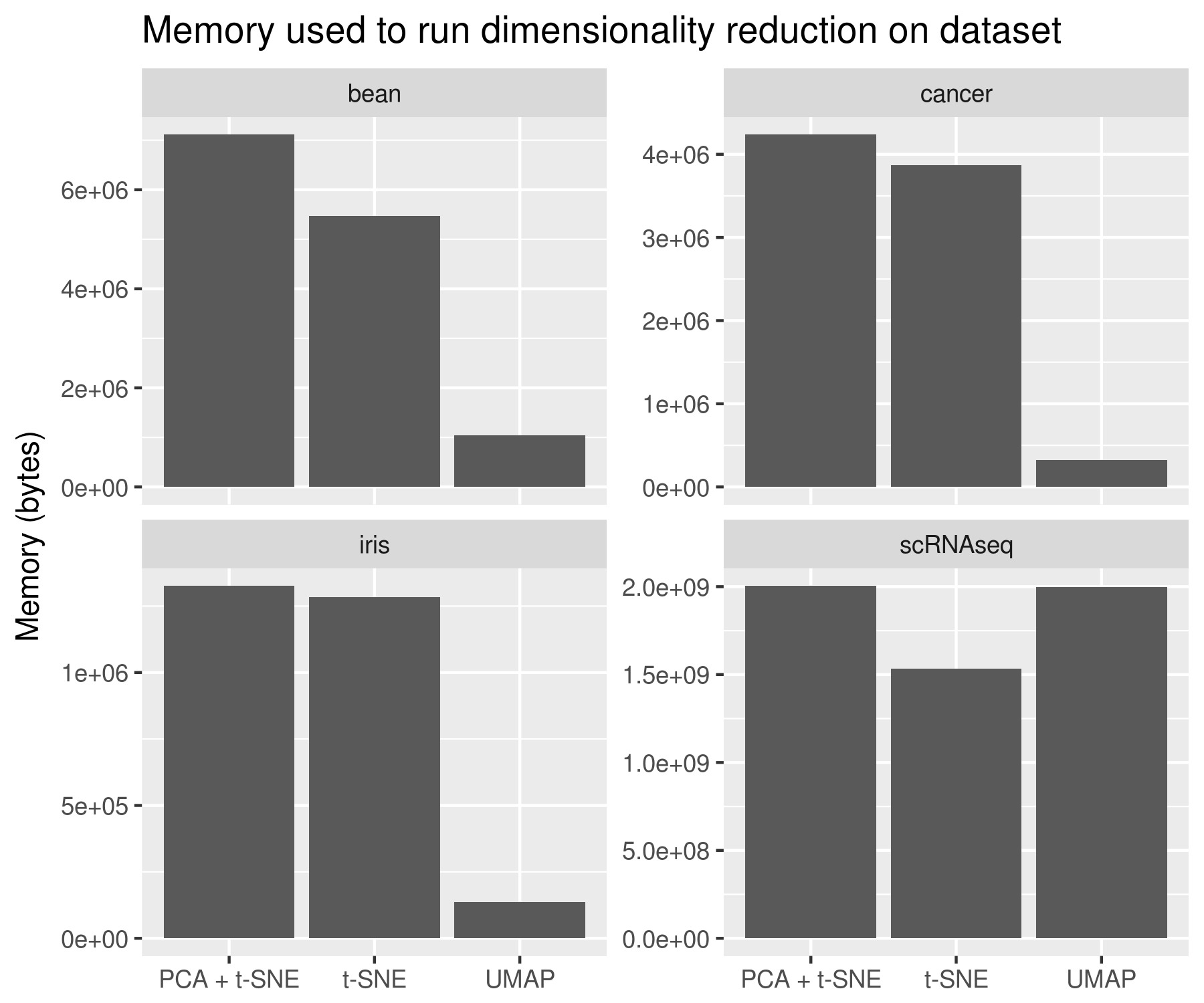
We compared UMAP to PCA and t-SNE alone, as well as to t-SNE run on data preprocessed with PCA. In each case, the data were subset to include only complete observations. The code to reproduce these findings are available in timings.R.

The first data set is the same iris data set used above (149 observations of 4 variables):

Next we tried a cancer data set, made up of 699 observations of 10 variables:

Third we tried a soybean data set. It is made up of 531 observations and 35 variables:

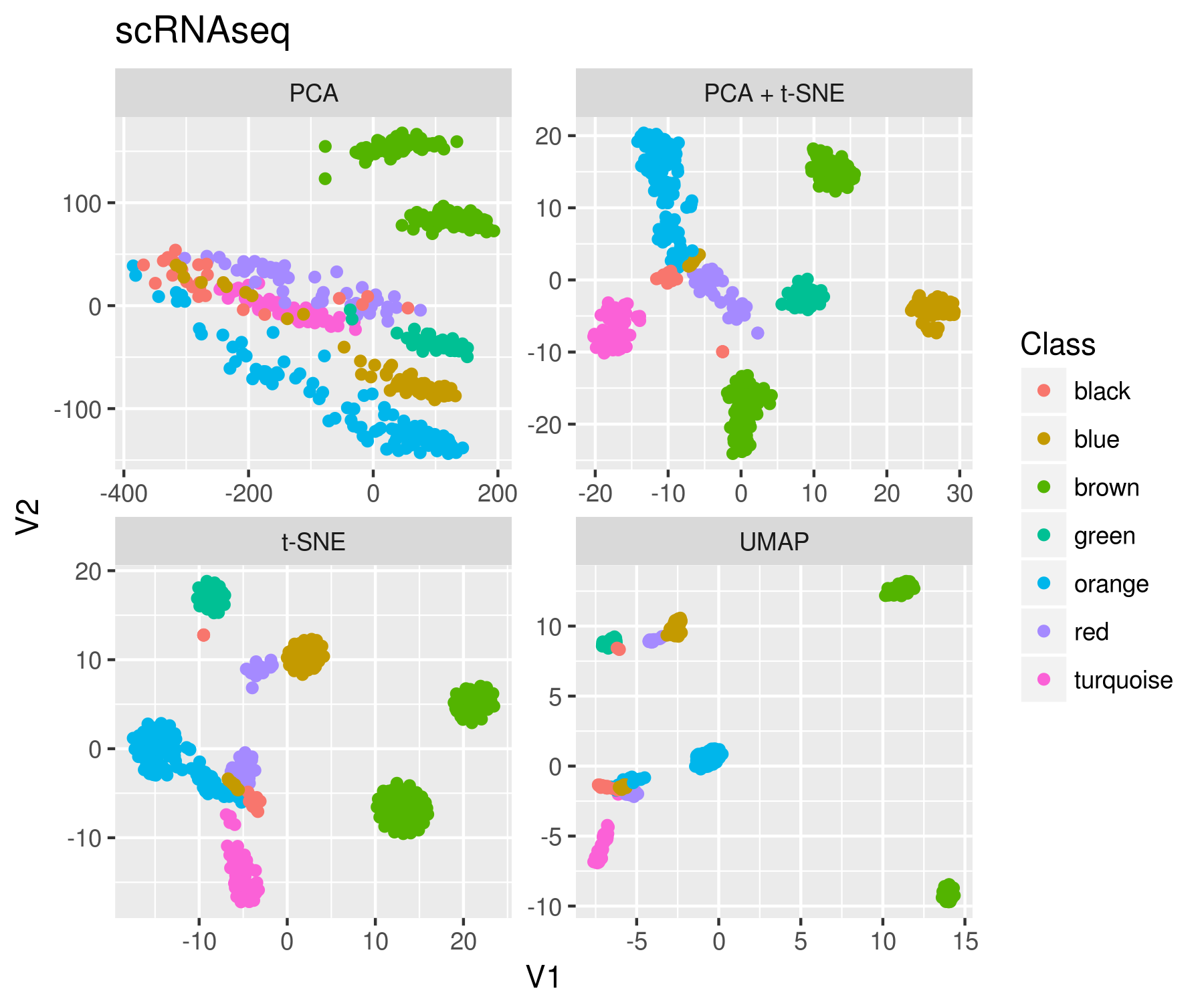
Finally we used a large single-cell RNAsequencing data set, with 561 observations (cells) of 55186 variables (over 30 million elements)!

PCA is orders of magnitude faster than t-SNE or UMAP (not shown). UMAP, though, is a substantial improvement over t-SNE both in terms of memory and time taken to run.

Related projects

• umap: R implementation of UMAP
• seurat: R toolkit for single cell genomics
• smallvis: R package for dimensionality reduction of small datasets