Invariant Superpixel Features for Object Detection & Localization
by Sam Johnson
Introducing DSeg
DSeg is a novel superpixel-based feature designed to be useful in semantic segmentation, object detection, and pose-estimation/localization tasks. DSeg extracts the shape and color of object-positive and object-negative superpixels, and encodes this information in a compact feature vector.
While this project is only in its infancy, DSeg has already shown promising results on superpixel-wise object detection (is superpixel A part of an instance of object class B?). Below we cover the implementation details of DSeg, present preliminary experimental results, and discuss future work and additional enhancements.
Motivation
Many who work or dabble in computer vision have noticed the intrinsic, deep coupling between image segmentation and higher-level tasks, such as detection, classification, localization, or more generally, whole-image understanding. The interdependence between these crucial computer vision tasks and segmentation is undeniable, and often frustrating. A chicken-and-egg scenario quickly arises:
How can you properly find the outline of an object without knowing what it is?
On the other hand, how can you begin to understand the context and identity of an object, before determining its extents?
Superpixel Segmentation
One "neat trick" that partially alleviates this issue is the superpixel segmentation algorithm. Superpixels arise from a clever, over-segmentation of the original image. Once the superpixel algorithm has been run, virtually all major and most minor edges and boundaries in the image will fall on some boundary or another between two superpixels. This fact exposes an intriguing trade-off: after running the superpixel algorithm, we can rest assured that virtually all edges and boundaries of interest have been found somewhere encoded in our superpixels. That said, we unfortunately also have to deal with a large number of minor or imagined edges that are included in the superpixel segmentation.
Properties of Superpixels
Superpixels are extremely powerful because they often fall on important boundaries within the image, and tend to take on abnormal or unique shapes when they contain salient object features. For example, in the superpixel segmentation of the below aircraft carrier, notice that the most salient object features (the radar array, anchor, and railing of the carrier) are almost perfectly segmented by highly unique superpixels.

Fig. 1: A superpixel segmented aircraft carrier. Salient features are revealed by the superpixels.
From this example, several intuitions arise:
- In general, superpixels tend to hug salient features and edges in the image
- "Weird" superpixels that differ greatly from the standard hexagonal (or rectangular) shape are more likely to segment points of interest
- "Boring" superpixels are part of something larger than themselves, and can often be combined with adjacent superpixels
Advantages of Synthetic Data
When writing object detectors, it helps to have images that fully describe the broad range of possible poses of the object in question. With real-world images, this is seldom possible, however the advent of readily available, high quality 3D models, and the maturity of modern 3D rendering pipelines has created ample opportunity to use synthetic renderings of 3D models to generate training data that:
- Covers the full range of poses of the object in question, with the ability to render arbitrary poses on the fly
- Can be tuned to vary scale, rotation, translation, lighting settings, and even occlusion
- Is already segmented (at every possible pose) without the need for human labeling
- Is easy to generate, no humans required once a 3D model is made

Fig. 2: 3D rendering of a Hamina-class missile boat, one of the models used to train DSeg
DSeg Feature Extraction Pipeline
In this section we outline the details of the DSeg feature extraction pipeline and comment on the major design decisions and possible future work and/or alterations.
Image Data Sources
DSeg requires a synthetic data source (i.e. a 3D model of the object that is to be learned) to generate class-positive training samples, and a "real-world" image source, preferably scene images, to generate class-negative training samples. That is, we use synthetic data to generate positive examples of our object class's superpixels, and we use real-world data to generate negative examples of our object class's superpixels.
For this project, we used the high quality ships 3D model dataset from [1], and SUN2012 [2] for real-world scene images. In particular, we randomly sampled 2000 images from [2], and for each 3D model in [1], we rendered 27,000 auto-scaled, auto-cropped poses uniformly distributed across the space off possible poses at 128 x 128, at a fixed camera distance, and with slightly variable lighting. The rendering of these images is covered in greater depth in [1].
DSeg Step 1: Segmentation
SLIC [3] is the state-of-the-art method for performing superpixel segmentation, whereas gSLICr [4] is a CUDA implementation of SLIC that can perform superpixel segmentation at over 250 Hz. Ideally we would use gSLICr in our pipeline, however significant modifications would need to be made to gSLICr to make it possible to extract the pixel boundaries of the generated superpixels, so we settled on the slower, VLFeat [5] implementation of SLIC.
We run SLIC on each image in our training set with a constant regularization parameter of 4000 (so as to avoid over-sensitivity to illumination). We do this over a range of 25 different grid sizes to ensure we capture all of the possible superpixel shapes that could occur within our object (or couldn't occur, in the case of negative examples). For positive examples, it is necessary to ignore superpixels that are not part of the object, however this is easy since we rendered translucent PNGs and merely need to ignore superpixels with transparent pixels.

Fig. 3: Superpixel segmentation is performed at multiple scales
For each valid superpixel found in the current image, we will eventually create a feature vector. Before passing these superpixel features on to the next pipeline stage, we calculate the closest-to-average RGB color for each superpixel. That is, we calculate for each superpixel the RGB color from its color palette that is closest to the mean RGB color across the entire superpixel. We measure color distance simply using the 3D euclidean distance formula. Future work might explore LAB or other color spaces.
In practice, stage 2 yields approximately 700 features per positive input image, depending on the model and viewing angle.
DSeg Step 2: Scale Invariance via ResizeContour
To obtain scale invariance for our features, we must normalize all of our superpixel features to the same square grid size. For this project, we used a 16 x 16 pixel grid.
A naive approach to this normalization phase would be to use an off-the-shelf image re-sizing routine, such as bicubic or bilinear interpolation. In practice, we found that these algorithms, along with nearest neighbor and other alternatives all result in either excessive blurring or pixelation when up-scaling very small features (which are quite common in DSeg, as most features are approximately 6 x 6 pixels in size. This blurring or pixelation means that a neural network will be able to tell that the feature in question was up-scaled. The purpose of scale invariance is to hide all evidence that any sort of up-scaling or down-scaling has taken place, so this is undesirable.

*Fig. 4: comparison of image re-sizing algorithms up-scaling from 16x16
ResizeContour
ResizeContour is a simple, novel algorithm for up-scaling single color threshold images with neither the pixelation introduced by nearest neighbor, nor the blurring introduced by bilinear interpolation. ResizeContour is how we up-scale superpixels (especially very small ones) in DSeg. The algorithm itself is relatively simple:
- Project each pixel from the original image to its new location in the larger image
- Find all the black (filled in) pixels among the 8 pixels immediately surrounding our pixel in the original image
- Project the coordinates of these dark pixels to the new larger image
- Perform a polygon fill operation using this list of projected points

Fig. 5: ResizeContour in action. The + signs represent pixels from the original superpixel.
Because we fill in overlapping polygons over each pixel in the image, this approach will only work if the entire image is of one uniform color. A side effect of this algorithm is that one pixel lines are usually erased from the resulting image, however this is good as it makes our features more block-like and more resistant to artifacts in the pre-segmented image.
Once the superpixel is re-sized to our decided canonical form, our feature vector is ready. We store the thresholded values of the pixel grid, concatenated with three floats representing the RGB value of the closest-to-average color. For a 16 x 16 standard superpixel size, this results in a 16 * 16 + 3 = 259 dimensional vector.
Evaluation
To evaluate the efficacy of DSeg as a general purpose feature, we constructed a simple experiment that trains (using RPROP) a standard feed-forward Multi-Layer Perceptron to take a single DSeg feature as input and output a single value indicating either that the feature belongs to an instance of our object, or that it is background noise and/or part of an unknown object. We conducted this same experiment on each of the 7 models used in RAPTOR (here) and observed slight variations in performance.
Network Topology
For our neural network, we used OpenCV's Multi-Layer Perceptron implementation. We used the recommended settings for Resilient Backpropagation (RPROP), which is known to converge more quickly than standard backpropagation, and has much fewer free parameters that need to be configured.
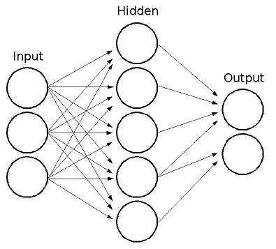
Input Layer
For input data, we used the formulation discussed earlier, generating features from our 27,000 positive input examples, and generating features from 2,000 negative input examples randomly selected from SUN2012. When a feature is sent to our neural network, it is processed as a 259-dimensional vector of floats, where the input grid is represented as 0.0's and 1.0's, and the RGB color is represented as three floats. Because of the inordinate number of features generated by this procedure, we randomly selected 500,000 features from the input set, and trained off of these. We used a 50/50 negative/positive example split. We also utilized a separate validation set roughly 1/2 the size of our training set.
Hidden Layer
We found that a hidden layer consisting of 48 neurons was sufficient. While we experimented with networks with many more neurons (and hidden layers), none seemed to have any advantage over our 48 hidden neuron setup. For an activation function throughout the network, we used the classic hyperbolic tangent function.
Output Layer
We used a single output neuron, where a value less than 0.5 indicates the input was not of our object class, and a value of 0.5 or greater indicates the input was of our object class.
Results
The table below displays the accuracy results for the best network we were able to train for each of the 7 RAPTOR models, including the model name, number of training epochs, and accuracy (based off of the validation set).
| Model | Training Epochs | Accuracy |
|---|---|---|
| Hamina | 140 | 72.24% |
| Halifax | 189 | 69.98% |
| Kirov | 137 | 71.31% |
| Kuznet | 162 | 70.12% |
| SovDDG | 145 | 65.7% |
| Udaloy | 80 | 70.17% |
| M4A1 | 153 | 71.5% |
Most models were able to yield 70% accuracy or nearly 70% accuracy. It is no surprise that the Hamina missile boat performed the best, as of all the models it has the highest number of visually recognizable features, and is not as oblong as the other models. The M4A1 is the only model in the set that is not a ship (it is, in fact, an assault rifle). It was our second best performing model, most likely due to its easily recognizable shape and correspondingly unique superpixel shapes.
Given that we used a simple Multi-Layer Perceptron, it is striking that we were able to achieve even 70% accuracy for a task as difficult as per-superpixel object classification.
Future Work
Follow-up studies must be conducted to continue to verify the efficacy of DSeg as a multi-purpose feature vector. In particular, it will be important to benchmark DSeg as a feature in deep networks that perform object detection and/or localization.
A very valuable study that could be conducted would be to generate DSeg features for objects in MS COCO, and supplement this data with synthetic data rendered from 3D models of common objects in COCO. This would allow us to benchmark DSeg against a commonly used dataset.
Performing classification based on a single superpixel feature is extremely difficult. Perhaps an easier (but more difficult to design) experiment would be to create a network that takes as input a DSeg superpixel feature, augmented by features for the top 5 nearest superpixels. The network would be trained to determine the object classification of the middle superpixel, and this would be significantly easier because it would have context information in the form of the surrounding superpixels.
Installation
DSeg has only been tested on Ubuntu 14.04. To install, do the following:
- Make sure you have CUDA installed and available (visit [https://developer.nvidia.com/cuda-downloads]
(https://developer.nvidia.com/cuda-downloads) for more info. - Clone the DSeg repo
git clone [email protected]:samkelly/DSeg.git cdinto the local repo./install_prerequisites.sh
You can now run the "delvr" command-line utility via ./build_run.sh. You can customize
build_run.sh to carry out various DSeg related tasks (see commented out lines for examples).
Related Work
Of particular importance to this project are the original SLIC superpixel segmentation routine [3], gSLICr [4], the state-of-the-art CUDA implementation of SLIC, as well as VLFeat [5], OpenCV [6], and the Boost C++ library [7].
The authors of [6] derive a fully convolutional model capable of semantic segmentation. As with DSeg, their network performs superpixel-wise classification, resulting in fully segmented object proposals. Unlike DSeg, their network can analyze an entire image rather than one superpixel at a time, but as a result, their approach is more of an end-to-end detection and segmentation solution than a feature extraction pipeline that might be of some help to high level computer vision tasks.
In [8], the authors leverage a similar synthetic data scheme whereby commodity 3D models are used to augment and/or replace real-world images in lieu of sufficient training data. This idea first appeared in the 2014 RAPTOR technical report [1], from which this project originally evolved.
References
-
Sam Kelly, Jeff Byers, David Aha, "RAPTOR Technical Report", NCARAI Technical Note, Navy Center for Applied Research in Artificial Intelligence. September 2014.
-
J. Xiao, J. Hays, K. Ehinger, A. Oliva, and A. Torralba. "SUN Database: Large-scale Scene Recognition from Abbey to Zoo", IEEE Conference on Computer Vision and Pattern Recognition, 2010.
-
Radhakrishna Achanta, Appu Shaji, Kevin Smith, Aurelien Lucchi, Pascal Fua, and Sabine S`usstrunk, "SLIC Superpixels", EPFL Technical Report 149300. June 2010.
-
Carl Yuheng Ren, Victor Adrian Prisacariu, and Ian D Reid, "gSLICr: SLIC superpixels at over 250Hz", ArXiv e-prints, 1509.04232. September 2015.
-
"VLFeat", http://ivrl.epfl.ch/research/superpixels
-
"OpenCV", http://opencv.org/
-
"Boost C++ Libraries", http://boost.org
-
Jonathan Long, Evan Shelhamer, and Trevor Darrell. "Fully convolutional networks for semantic segmentation." Proceedings of the IEEE Conference on Computer Vision and Pattern Recognition. 2015.
-
Xingchao Peng, Baochen Sun, Karim Ali, Kate Saenko, "Learning Deep Object Detectors from 3D Models", ArXiv e-prints, 1412.7122v4. October 2015.