ggdistribute

A ggplot2 Extension for Plotting Unimodal Distributions

The ggdistribute package is an extension for plotting posterior or other types of unimodal distributions that require overlaying information about a distribution’s intervals. It makes use of the ggproto system to extend ggplot2, providing additional “geoms”, “stats”, and “positions.” The extensions integrate with existing ggplot2 layer elements.

Example

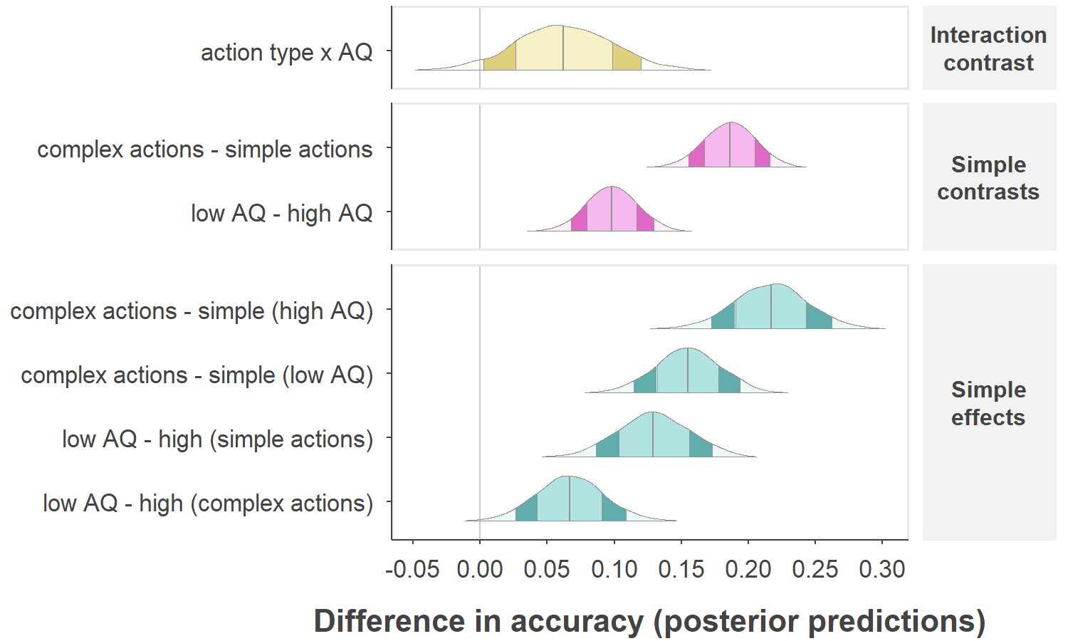
The package function example_plot() is an overview of combining ggdistribute with other ggplot2 elements. The contents of this function are printed below and gives details about the extended parts to ggplot2.

library(ggplot2)
library(ggdistribute)

example_plot <-
function() {
  # color palette
  colors <- mejr_palette()

  ggplot(sre_data(5000), aes_string(y="effect")) +

    # ggdistribute specific elements -------------------------------------------
    geom_posterior(
      # ~~~~~~~~~~~~~~~~~~~~~~~~~~~~~~~~~~~~~~~~~~~~~~~~~~~~~~~~~~~~~~~~~~~~~~~~
      # geom_posterior() aesthetics mappings
      # ~~~~~~~~~~~~~~~~~~~~~~~~~~~~~~~~~~~~~~~~~~~~~~~~~~~~~~~~~~~~~~~~~~~~~~~~
      aes_string(x="value", fill="contrast"),
      # ~~~~~~~~~~~~~~~~~~~~~~~~~~~~~~~~~~~~~~~~~~~~~~~~~~~~~~~~~~~~~~~~~~~~~~~~
      # options passed to stat_density_ci() for estimating intervals
      # ~~~~~~~~~~~~~~~~~~~~~~~~~~~~~~~~~~~~~~~~~~~~~~~~~~~~~~~~~~~~~~~~~~~~~~~~
      interp_thresh=.001, # threshold for interpolating segment gaps
      center_stat="median", # measure of central tendency
      ci_width=0.90, # width corresponding to CI segments
      interval_type="ci", # quantile intervals not highest density interval
      # ~~~~~~~~~~~~~~~~~~~~~~~~~~~~~~~~~~~~~~~~~~~~~~~~~~~~~~~~~~~~~~~~~~~~~~~~
      # options passed to stat_density_ci() for estimating density
      # ~~~~~~~~~~~~~~~~~~~~~~~~~~~~~~~~~~~~~~~~~~~~~~~~~~~~~~~~~~~~~~~~~~~~~~~~
      bw=".nrd0", # bandwidth estimator type
      adjust=1.5, # adjustment to bandwidth
      n=1024, # number of samples in final density
      trim=.005, # trim `x` this proportion before estimating density
      cut=1.5, # tail extension for zero density estimation
      # ~~~~~~~~~~~~~~~~~~~~~~~~~~~~~~~~~~~~~~~~~~~~~~~~~~~~~~~~~~~~~~~~~~~~~~~~
      # geom_posterior() options
      # ~~~~~~~~~~~~~~~~~~~~~~~~~~~~~~~~~~~~~~~~~~~~~~~~~~~~~~~~~~~~~~~~~~~~~~~~
      draw_ci=TRUE, # toggle showing confidence interval parts
      draw_sd=TRUE, # toggle showing standard deviation parts
      mirror=FALSE, # toggle horizontal violin distributions
      midline=NULL, # line displaying center of dist. (NULL=aes color)
      brighten=c(3, 0, 1.333), # additive adjustment of segment fill colors
      # ~~~~~~~~~~~~~~~~~~~~~~~~~~~~~~~~~~~~~~~~~~~~~~~~~~~~~~~~~~~~~~~~~~~~~~~~
      # position_spread() options
      # ~~~~~~~~~~~~~~~~~~~~~~~~~~~~~~~~~~~~~~~~~~~~~~~~~~~~~~~~~~~~~~~~~~~~~~~~
      position=position_spread(
        reverse=TRUE, # order of spreaded groups within panels
        padding=0.3, # shrink heights of distributions
        height="panel" # scale by heights within panels
      ), #
      # ~~~~~~~~~~~~~~~~~~~~~~~~~~~~~~~~~~~~~~~~~~~~~~~~~~~~~~~~~~~~~~~~~~~~~~~~
      # standard ggplot layer options
      # ~~~~~~~~~~~~~~~~~~~~~~~~~~~~~~~~~~~~~~~~~~~~~~~~~~~~~~~~~~~~~~~~~~~~~~~~
      size=0.15, color=colors$gray, vjust=0.7, show.legend=FALSE
    ) +

    # standard ggplot2 elements ------------------------------------------------
    geom_vline(alpha=0.5, color=colors$gray, size=0.333, linetype=1, xintercept=0) +
    scale_x_continuous(breaks=seq(-1, 1, .05)) +
    facet_grid("contrast ~ .", scales="free_y", space="free_y") +
    scale_fill_manual(values=c(colors$yellow, colors$magenta, colors$cyan)) +
    labs(x="Difference in accuracy (posterior predictions)") +
    theme(
      legend.position="none", strip.text.y=element_text(angle=0, hjust=0.5),
      panel.border=element_rect(fill=NA, color=colors$lightgray, size=0.67),
      panel.grid=element_blank(), panel.ontop=FALSE, axis.title.y=element_blank(),
      plot.margin=margin(t=2, r=4, b=2, l=2, unit="pt")
    )
}

Additional examples from an arbritrary dataset

# total number of samples in the dataset
N <- 2500
means <- c(-1, 2, 3, 5)

The data object below is a randomly generated dataset of 4 different normal distributions. Two factors, Condition and Group, are assigned to subsets of the generated values. 2500 samples are generated for each value of mu for a total of $ 10^{4} $ rows.

data <- data_normal_sample(mu = means, n = N)

Create a new grouping variable called Level based on the column Group.

# number of levels to make
num_levels <- 8L

# R version >= 3.5 now let's you assign factors this way.
data$Level <- with(data, factor(
  Group,
  levels = letters[seq_len(num_levels)],
  labels = c(rep("Low", 3), rep("Mid", 2), rep("High", 3)),
  ordered = TRUE
))

Show unique groups per Group, Condition, and Level to help understand the data factors.

unique(data[, c("Group", "Condition", "Level")])
#> # A tibble: 8 x 3
#>   Group Condition Level
#>   <chr> <chr>     <ord>
#> 1 a     A         Low  
#> 2 b     A         Low  
#> 3 c     B         Low  
#> 4 d     B         Mid  
#> 5 e     C         Mid  
#> 6 f     C         High 
#> 7 g     D         High 
#> 8 h     D         High

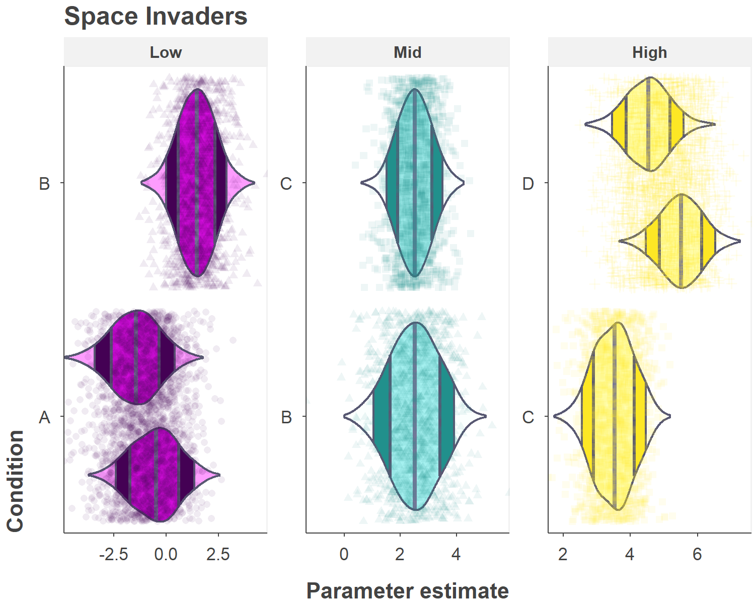
Facetting and spreading groups

ggplot(data) +
  aes(x=value, y=Condition, group=Group) +
  geom_posterior(
    aes(fill=Level),
    mirror=TRUE,
    show.legend=FALSE,
    adjust=1.5,
    brighten=c(6, 0, 2.5),
    position=position_spread(reverse=TRUE)
  ) +
  geom_point(
    aes(color=Level, shape=Condition),
    alpha=.08,
    fill=NA,
    show.legend=FALSE,
    position=position_jitter(0, .45)
  ) +
  coord_cartesian(ylim=c(0.5, 2.5), expand=FALSE) +
  facet_wrap(~ Level, scales="free") +
  labs(title="Space Invaders", y="Condition", x="Parameter estimate")

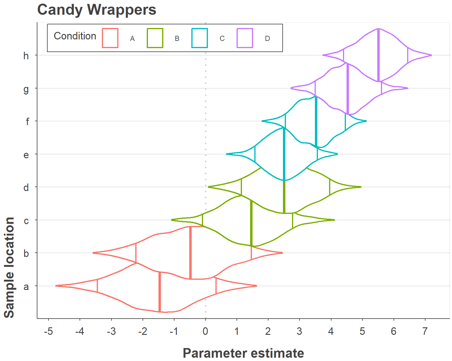
Changing the appearance of geom_posterior

ggplot(data) +
  aes(x=value, y=Group) +
  geom_vline(
    xintercept=0, size=.6
  ) +
  geom_posterior(
    aes(color=Condition),
    midline=NULL,
    mirror=TRUE,
    fill="#FFFFFF",
    draw_sd=FALSE,
    interval_type="hdi",
    vjust=0,
    position=position_spread(height=2)
  ) +
  labs(
    title="Candy Wrappers",
    x="Parameter estimate",
    y="Sample location"
  ) +
  scale_x_continuous(breaks=seq(-10, 10, 1)) +
  theme(
    legend.position=c(.025, .9),
    legend.justification=c(0, 0),
    panel.grid.major.y=element_line(color=gray(.92))
  )

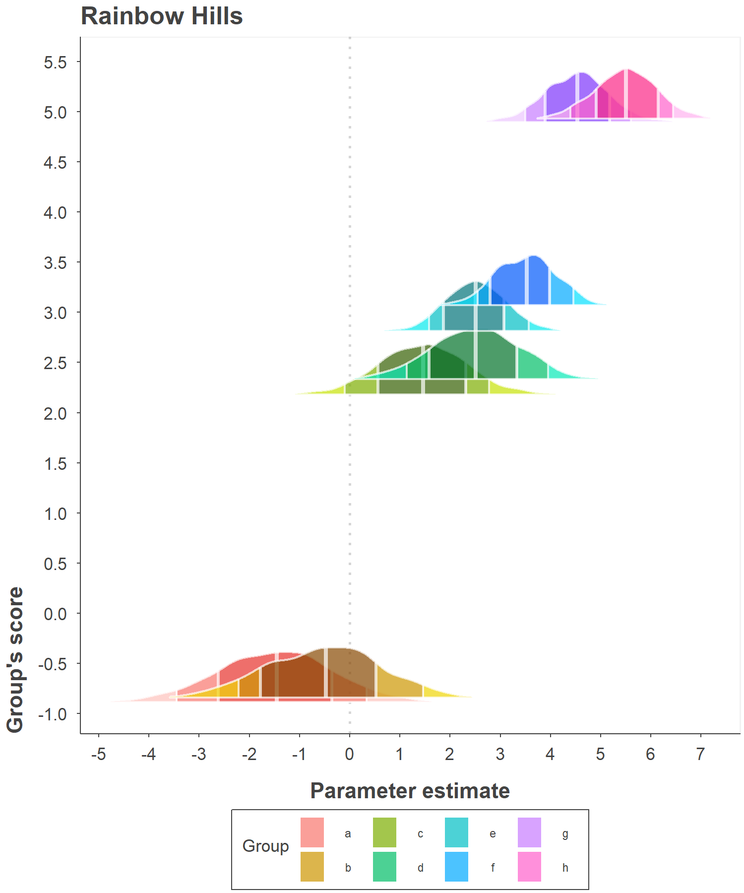
The y axis is a repeated, continuous grouping variable

The variable GroupScore is a continuous variable assigned to each Group. The distributions will be positioned at the start of the y value for each group, and resized to not overlap with the next group. Resizing can be overriden by specifying height in position_spread.

unique(data[, c("Group", "GroupScore")])
#> # A tibble: 8 x 2
#>   Group GroupScore
#>   <chr>      <dbl>
#> 1 a         -0.885
#> 2 b         -0.839
#> 3 c          2.18 
#> 4 d          2.33 
#> 5 e          2.81 
#> 6 f          3.07 
#> 7 g          4.90 
#> 8 h          4.93

ggplot(data) +
  aes(x=value, y=GroupScore) +
  geom_vline(
    xintercept=0, size=.6
  ) +
  geom_posterior(
    aes(fill=Group),
    midline="#FFFFFF",
    colour="#FFFFFF",
    alpha=0.7,
    brighten=c(1.3, 0, -1.3),
    interval_type="hdi",
    position=position_spread(height=0.5, padding=0)
  ) +
  labs(
    title="Rainbow Hills",
    x="Parameter estimate",
    y="Group's score"
  ) +
  scale_x_continuous(breaks=seq(-10, 10, 1)) +
  scale_y_continuous(breaks=seq(-10, 10, .5))

How to install

Dependencies

• R: https://www.r-project.org/

A current R installation.

Dependencies for installing the development version of this package

• devtools package: https://www.rstudio.com/products/rpackages/devtools/

The devtools package is an R package that makes it easier to install local or remote content as an R package that can be used like any other standard R package. You can install devtools by opening up RStudio or an R terminal and running

install.packages("devtools")

For Windows users, you may be required to install Rtools first before you can use the devtools package, if there is any code that needs to be compiled. These are a set of build tools customized for building R packages (see the devtools link above for more details).

• Build tools: http://cran.r-project.org/bin/windows/Rtools/

Installing from CRAN

If you want to use the last version that was uploaded to the CRAN repository, do the following:

install.packages("ggdistribute")

Installing from the downloaded package content folder

If you have all of the ggdistribute package contents (e.g., an unzipped folder containing DESCRIPTION, NAMESPACE, R/, etc…), you can open up the ggdistribute.Rproj file in RStudio and use both devtools and RStudio to load or install package.

The first step is to make sure you have all the package dependencies (other packages that this pacakge relies on) to be able to load or install the ggdistribute package materials. You can run the line below to install dependencies first.

devtools::install_dev_deps()

After the dependencies are installed, you can now build and install ggdistribute from the current working directory. Assuming the ggdistribute project is loaded in RStudio, you can leave out the first argument.

devtools::install()

If installing from a different working directory, enter the path of the package contents to manually specify what to install.

devtools::install_dev_deps("/Path/to/the/folder/ggdistribute")
devtools::install("/Path/to/the/folder/ggdistribute")

Installing from GitHub

If devtools are installed, you may use the install_github() function to download and install the development version of the package from this GitHub repository instead of the one hosted on CRAN. Run the code below to download and install the development version:

devtools::install_github("iamamutt/ggdistribute")

or to install all suggested packages as well…

devtools::install_github("iamamutt/ggdistribute", dependencies=TRUE)

Loading the package

If successful, the package should now be installed and can be loaded as any other package. Repeat the last intall step if there are updates to the package, or complete all steps to install on another machine. You should now be able to use the package materials and should see it in your packages tab if using RStudio. It should be loaded like any other package.

library(ggdistribute)

Getting help

Browsing the vignettes

Vignettes can be viewed in several different ways.

• pre-built and saved in the inst\doc folder on GitHub.
• calling vignette("geom_posterior", "ggdistribute") from within R after the package is installed.
• navigating to packages tab > ggdistribute > User guides, package vignettes… in RStudio.

Viewing the help documentation

View the package welcome page to navigate to different types of help documents

package?ggdistribute

Viewing package information and a list of exported objects:

help(package = "ggdistribute")

# or
library(help="ggdistribute")