Kubeflow - Data Science on Steroids

Welcome to the blog post and corresponding talk about Kubeflow. This is a project of mbu93 and saschagrunert. Feel free to open issues if you have questions or want to provide feedback to us.

You can find the blog post:

• within this repository
• on SUSE
• on Medium

The corresponding talk can be found:

• on Meetup

The slides of the talk:

• on Slides.com

Table of Contents

• About
• Data Science on Steroids with Kubeflow
  • The Evolution of Machine Learning
  • The Classic Data Science Workflow
  • Yet Another Machine Learning Solution?
    • Kubernetes and Cloud Native Applications
    • Kubeflow to the Rescue
  • The Deployment and Test Setup
    • Kubernetes
    • Storage Provisioner
    • Load Balancing
    • Deploying Kubeflow
  • Improving the Data Scientists Workflow
    • Cloud Native Notebook Servers
    • Machine Learning Pipelines
    • Machine Learning Pipelines within Notebooks
    • Continuous Integration Lookout
  • Conclusion

About

Artificial intelligence, machine and deep learning are probably the most hyped topics in software development these days!

New projects, problem solving approaches and corresponding start-ups pop up in the wild on a daily basis. Most of the time, the major target is to get an understandable output from a huge set of unmanageable input data. To achieve this goal, the in fact standard frameworks TensorFlow and PyTorch established a rich set of features over time by being well maintained under the hood, too. But the simple usage of these frameworks does not solve today’s software related challenges like continuous integration (CI) and deployment (CD). The creation of a sustainable workflow, which embeds seamlessly into the existing infrastructure as well as existing CI/CD pipelines, are one of the major obstacles software developers are facing today.

Another trend related to this topic is the increasing usage of Kubernetes as build and test infrastructure for on premise and managed cluster architectures. But how to utilize the full power of Kubernetes-based cloud environments, when it comes to training and deploying machine learning models? How to integrate them into existing continuous integration and deployment pipelines? Can we split up machine learning workflows into separate pipeline steps, like we already do within our existing CI/CD setups?

In this talk and corresponding blog post we will discover the possibilities to utilize the joint forces of Kubernetes and Data Science. For this we have chosen to elaborate Kubeflow, one of the most common open source cloud native platforms for machine learning.

Kubeflow is a project which is dedicated to making deployments of machine learning workflows on Kubernetes simple, portable and scalable. It is a relatively young project which aims to provide a complete machine learning toolkit on top of Kubernetes.

Join us and we will discover the exciting features of Kubeflow together, like spawning and managing Jupyter servers and creating our very own machine learning pipelines from scratch.

Data Science on Steroids with Kubeflow

Before we dive into the cloud native topics and Kubeflow, let’s just have a look back at the history of machine learning and artificial intelligence at all.

The Evolution of Machine Learning

Machine learning has its origins in the early 1950s, where the first machines like the Stochastic Neural Analog Reinforcement Calculator (SNARC) Maze Solver appeared in the wild. The SNARC machine is known as the first Artificial Intelligence (AI) neural network ever built and it already contained synapses which were capable of storing their result in some kind of internal memory.

But let’s fast forward to the early 2000s, where the industry created the first software based machine learning frameworks which should revolutionize the world of computing. Torch, one of the first software libraries built for machine learning, was initially released in 2002. Other more on scientific computing specialized frameworks like NumPy were created around 2006, and a massive flood of machine learning tools and frameworks were released since then. TensorFlow, PyTorch and Pandas are only some of the big players in machine learning today. Most of these frameworks are built to be used from the Python programming language, which itself gained a massive boost regarding its popularity because of this booming industry around artificial intelligence.

The multi-disciplinary field of Data Science utilizes the methods of machine learning as well as their rich tooling landscape to solve problems from the statistical perspective. But what are these guys really doing from day to day and how does their workflow currently look like?

The Classic Data Science Workflow

First of all, we have to mention that there is no magic recipe when it comes to solving data scientific problems. Nevertheless, we still do similar steps in all these sorts of diverging solution approaches.

The source of the data to be analyzed is one common example. For sure, the input data will change over time, but the technology how to obtain these data mostly stays fixed. As a data scientist we also have no direct influence on this source. So for example, we could always use the latest database dump of the last week, which will produce different results over time. If the data got imported, we mostly process them via Python based Jupyter notebooks, to be able to annotate and layout our research approach even better.

Now that we have our data at hand, we have to decide which data exploration approach we’d like to use. We have to answer questions like “Do we need supervised or unsupervised learning?” and “Can we solve the problem with classification or regression?”. This for sure highly depends on the actual use case, but the common baseline is simply trying it out and building models around the different solution approaches. We call this step baseline modelling and use one of this powerful Python based machine learning frameworks out there. We can do this by not leaving the Jupyter notebook at all, which is pretty nice when working alone. But how to handle this when the problems get bigger and we have to collaborate with others? How to handle the resource limitations my workstation or the single remote server instance has?

Let’s skip the answers to these questions for now and follow up with the next step: The results communication. We now have a solution, a model which can be trained, and some first results to share. This is where it gets tricky sometimes. We have to choose a deployment method and find out how to update the model on a regular basis. The automatisms behind that are mostly custom solutions which fit on the single dedicated use case for what they are made for. If we don’t have a clear understanding of the infrastructure, then this part can get messy. Finding an automated way to process the input data from the database into a well-served resulting model gets even harder if the model has to be updated periodically.

Yet Another Machine Learning Solution?

So, there seems an already well established data science workflow and we have to ask ourself if we really want to have yet another machine learning solution in the wild. In our case, the answer is a big “YES”, because we know that the current situation is not satisfying at all. We want to choose a software solution which at least targets to solve all our main issues we had in the past, so why not choose something cloud native?

Kubernetes and Cloud Native Applications

The wording “cloud native” basically means that the applications run in container-based environments. But we have to distinguish between applications which are aware of running in a distributed system and those which are not. The latter are called commercially available of-the-shelf (COTS) applications, like a WordPress based blog. This application is fully controlled by its environment and has no direct influence on it. We call applications cloud native if they are aware that they run inside a distributed system like Kubernetes and utilize its API to modify anything within the cluster. These applications are on one hand much more powerful, but on the other hand less flexible when it comes to the deployment because they’re now bound to its target system.

To build a cloud native application, we have to split it up into microservices and maybe use modern software architectural approaches like service meshes. One of the most well-known approaches today is to use Kubernetes, which provides mainly all of the features we need to deploy a modern cloud native application.

The major question is now: “Can we improve the classic data scientists workflow by utilizing Kubernetes?”. We absolutely can! But Kubernetes alone won’t help us a lot, which means that we have to choose an appropriate cloud native solution on top, like the machine learning toolkit Kubeflow.

Kubeflow to the Rescue

Kubeflow has been announced around two years ago in 2017 with the main target to make machine learning stacks on Kubernetes easy, fast and extensible. The major goal of Kubeflow is to abstract machine learning best-practices, so that data scientists do not really need to understand what is happening in detail under the hood.

A lot of improvements happened to the project since its initial announcement, but in the end Kubeflow targets to be an umbrella project to close the gap between common use cases like running JupyterHub servers or deploying machine learning models based on TensorFlow or PyTorch. To do this, Kubeflow re-uses existing software solutions and wraps them in their own abstraction of a cloud native application by leveraging the features of Kubernetes.

Kubeflow today is a fast evolving project which has many contributors from the open source industry. Nevertheless, it aims to be an easy-to-use software project, which should also apply to the deployment of Kubeflow itself. But since it is using multiple software components, the overall deployment of Kubeflow is not that trivial as it may look like. This means we should spend some time to wrap our heads around the used test setup for the following demonstration purposes.

The Deployment and Test Setup

Please be aware that Kubeflow is a rapidly evolving software and the code examples may be out of date in the near future. If this is the case, feel free to reach out to me anytime. From now on we will focus on the latest available deployment strategy for bare metal or virtual machine (VM) based Kubernetes clusters. It is for sure possible to deploy Kubeflow on Google Cloud or Amazon Web Services, but this is out of scope of this blog post.

Kubernetes

First of all, we have to built up a Kubernetes cluster which fulfills a set of common requirements. To do this, we have chosen a beta of SUSE’s upcoming release of SUSE CaaS Platform, SUSE CaaS Platform 4. This comes with some well chosen components under the hood, like the CRI-O container runtime and Cilium for networking purposes. We utilized the new SUSE CaaS Platform bootstrapping tool skuba to rapidly set up an OpenStack based Kubernetes environment on top of four already existing SUSE Linux Enterprise Server 15 SP1 (SLES) machines.

We initialize the cluster under the current working directory:

> skuba cluster init --control-plane 172.172.172.7 caasp-cluster
> cd caasp-cluster

Then we bootstrap the master node:

> skuba node bootstrap --target 172.172.172.7 caasp-master

And now we join the three worker nodes:

> skuba node join --role worker --target 172.172.172.8  caasp-node-1
> skuba node join --role worker --target 172.172.172.24 caasp-node-2
> skuba node join --role worker --target 172.172.172.16 caasp-node-3

That’s it, with the usage of the automatically downloaded admin.conf we should be able to access the Kubernetes cluster:

> cp admin.conf ~/.kube/config
> kubectl get nodes -o wide
NAME           STATUS   ROLES    AGE  VERSION   INTERNAL-IP      EXTERNAL-IP   OS-IMAGE                              KERNEL-VERSION           CONTAINER-RUNTIME
caasp-master   Ready    master   2h   v1.15.2   172.172.172.7    <none>        SUSE Linux Enterprise Server 15 SP1   4.12.14-197.15-default   cri-o://1.15.0
caasp-node-1   Ready    <none>   2h   v1.15.2   172.172.172.8    <none>        SUSE Linux Enterprise Server 15 SP1   4.12.14-197.15-default   cri-o://1.15.0
caasp-node-2   Ready    <none>   2h   v1.15.2   172.172.172.24   <none>        SUSE Linux Enterprise Server 15 SP1   4.12.14-197.15-default   cri-o://1.15.0
caasp-node-3   Ready    <none>   2h   v1.15.2   172.172.172.16   <none>        SUSE Linux Enterprise Server 15 SP1   4.12.14-197.15-default   cri-o://1.15.0

The cluster is completely production ready and comes with strong security features like apparmor and pre-defined Pod Security Policies (PSPs).

Storage Provisioner

For running Kubeflow on top of our deployed cluster, we have to setup a Storage Provisioner, where we will use the Network File System (NFS) as underlying technology for sake of simplicity. Before setting up the provisioner, we install the nfs-client on all nodes for storage accessibility. We’d chose caasp-node-1 as NFS server, which needs some additional setup:

> sudo zypper in -y nfs-kernel-server
> sudo mkdir -p /mnt/nfs
> echo '/mnt/nfs *(rw,no_root_squash,no_subtree_check)' | sudo tee -a /etc/exports
> sudo systemctl enable --now nfsserver

This is for sure not production ready in terms of failure safety, but should be enough for our test setup. Now we can install the Kubernetes storage provisioner by using the latest pre-release of the package manager Helm 3, which comes without a server side deployment:

> helm install nfs-client-provisioner \
    -n kube-system \
    --set nfs.server=caasp-node-1 \
    --set nfs.path=/mnt/nfs \
    --set storageClass.name=nfs \
    --set storageClass.defaultClass=true \
    stable/nfs-client-provisioner

The storage provisioner should now be available up and running:

> kubectl -n kube-system get pods -l app=nfs-client-provisioner -o wide
NAME                                      READY   STATUS    RESTARTS   AGE   IP            NODE           NOMINATED NODE   READINESS GATES
nfs-client-provisioner-777997bc46-mls5w   1/1     Running   3          2h    10.244.0.91   caasp-node-1   <none>           <none>

Load Balancing

We also need a load balancer for accessing the cluster. For this we’d chose MetalLB, which works great with Cilium. To install it, we run:

> kubectl apply -f https://raw.githubusercontent.com/google/metallb/v0.8.1/manifests/metallb.yaml

Then we have to deploy a configuration, where we only need one single IP for accessing Kubeflow (172.172.172.251) later on:

> cat metallb-config.yml

---
apiVersion: v1
kind: ConfigMap
metadata:
  namespace: metallb-system
  name: config
data:
  config: |
    address-pools:
    - name: default
      protocol: layer2
      addresses:
      - 172.172.172.251-172.172.172.251

> kubectl apply -f metallb-config.yml

If you run MetalLB on OpenStack, please be aware that the networking has to be configured to allow IP spoofing to make the assigned IPs reachable.

Deploying Kubeflow

We utilize the Kubeflow internal deployment tool kfctl, which has been highly rewritten from scratch to replace a now deprecated shell script. The tool can consume multiple types of configurations, where we decided to choose the Arrikto configuration for vendor neutral authentication via Dex and Istio. It is worth to mention that there exists a new Istio based configuration, which should be free from any external dependencies, where the above mentioned load balancer would not be needed at all.

With an installed and up-to-date kfctl client, we’re now able to bootstrap the Kubeflow application into our Kubernetes cluster. First, we have to initialize the application:

> kfctl init kfapp --config=https://raw.githubusercontent.com/kubeflow/kubeflow/1fa142f8a5c355b5395ec0e91280d32d76eccdce/bootstrap/config/kfctl_existing_arrikto.yaml

Then we can set the default credentials for our testing purposes:

> export KUBEFLOW_USER_EMAIL="[email protected]"
> export KUBEFLOW_PASSWORD="my-strong-password"

And now install the application:

> cd kfapp
> kfctl generate all -V
> kfctl apply all -V

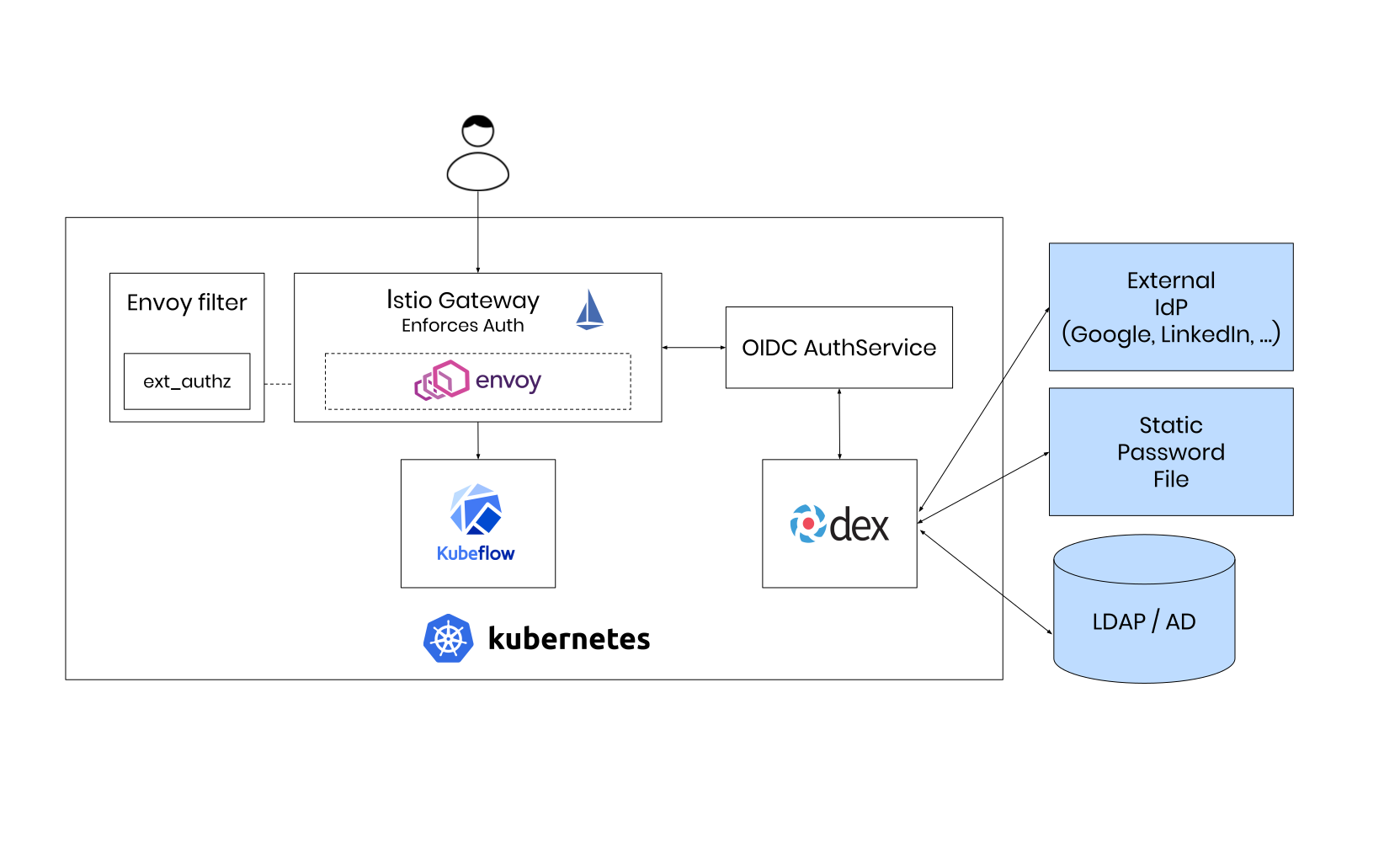
The overall architecture of the deployed application looks now like this, where we skipped the LDAP authentication part in replacement of the statically exported credentials.

Now, we should be able to access Kubeflow via the exposed IP of the Istio Gateway.

> kubectl -n istio-system get svc istio-ingressgateway
NAME                   TYPE           CLUSTER-IP       EXTERNAL-IP       PORT(S)                                                                                                                                                     AGE
istio-ingressgateway   LoadBalancer   10.102.112.227   172.172.172.251   5556:31334/TCP,15020:30057/TCP,80:31380/TCP,443:31390/TCP,31400:31400/TCP,15029:32004/TCP,15030:30908/TCP,15031:32568/TCP,15032:32127/TCP,15443:31037/TCP   4m23s

In our case, the problem is that our local machine is not part of the subnet where Kubernetes is deployed. But this obstacle can easily be overcome with a NAT redirection and by utilizing the possibilities of kube-proxy:

> sudo iptables -t nat -A OUTPUT -p all -d 172.172.172.251 -j DNAT --to-destination 127.0.0.1
> sudo kubectl -n istio-system port-forward svc/istio-ingressgateway 443 &
> kubectl -n istio-system port-forward svc/istio-ingressgateway 5556

If we now access https://localhost from our browser, then all traffic should be correctly routed to our local machine and after skipping the HTTPs security warnings the first login screen should appear:

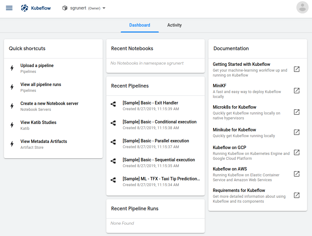
We can now authenticate with our pre-defined username and password. Here we are, welcome to the Kubeflow Central Dashboard:

Some first indicators already hint us to the fact that we’re running a cloud native application. For example, it looks like that Kubeflow created a Kubernetes namespace for us where we can work in. Let’s dive into the application itself since we finally have a working installation.

Improving the Data Scientists Workflow

Cloud Native Notebook Servers

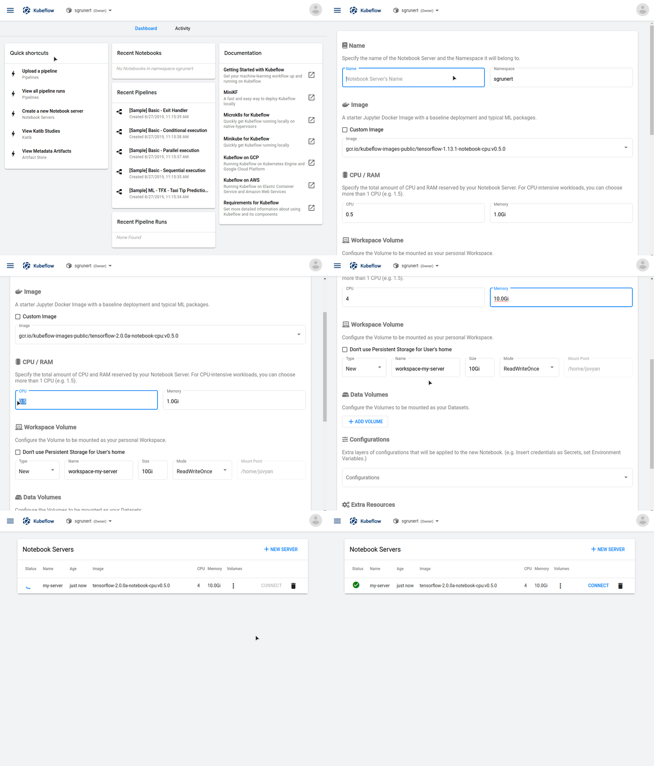
For example, with Kubeflow it is easily possible to create per-user Jupyter notebook servers:

This notebook server is now running as StatefulSet in the Kubernetes cluster within my personal namespace:

> kubectl -n sgrunert get pods,statefulsets
NAME              READY   STATUS    RESTARTS   AGE
pod/my-server-0   2/2     Running   0          3m7s

NAME                         READY   AGE
statefulset.apps/my-server   1/1     3m7s

We can also see that a persistent NFS storage has been provided for the notebook server as well:

> kubectl -n sgrunert get pvc
NAME                  STATUS   VOLUME                                     CAPACITY   ACCESS MODES   STORAGECLASS   AGE
workspace-my-server   Bound    pvc-cd92e3a5-0be4-4ced-af91-b15ac5601f9b   10Gi       RWO            nfs            4m38s

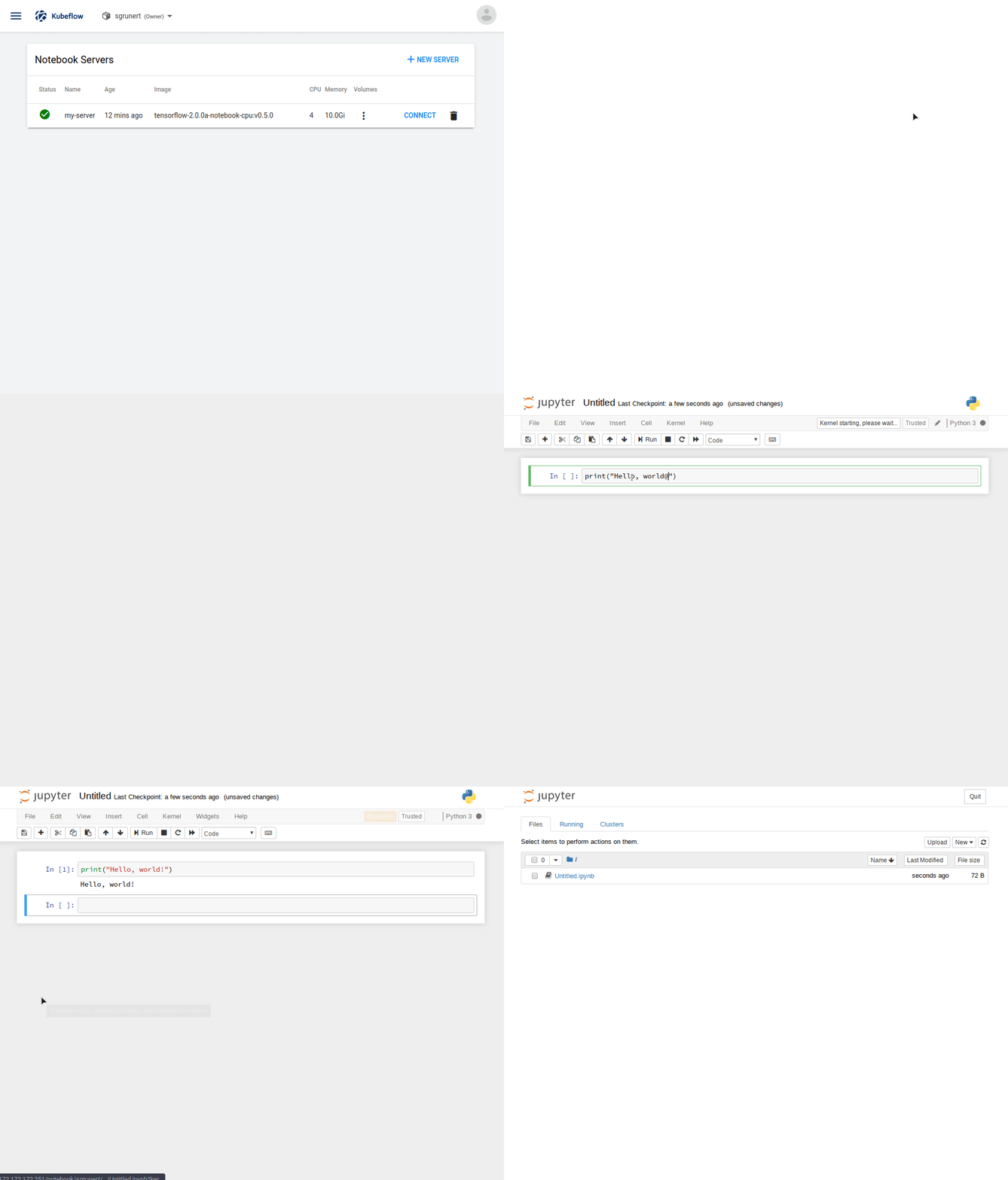
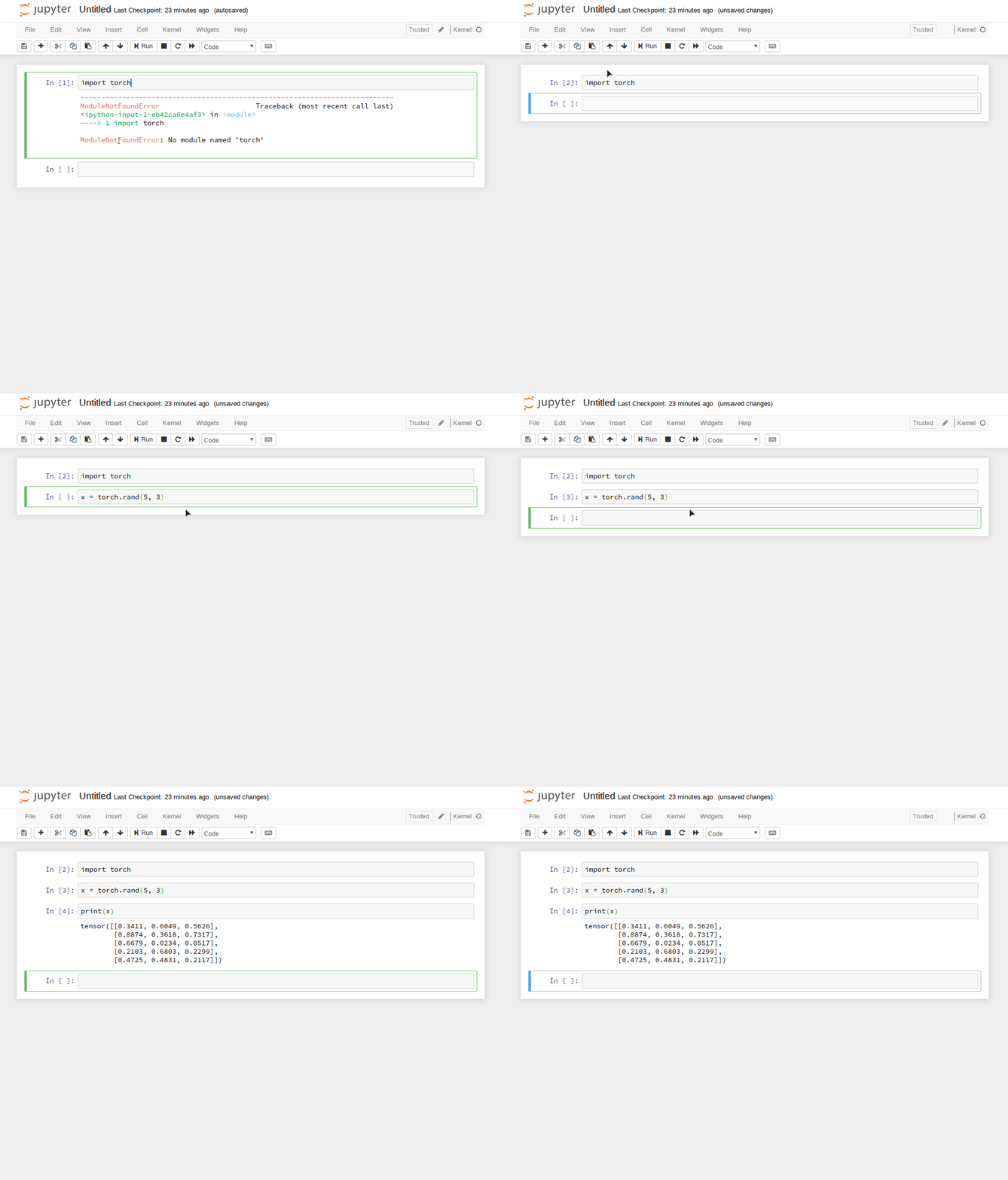
Let’s connect to the notebook server and test if it’s working as we would expect it:

Nice, this works like every other usual Jupyter Hub notebook. The major benefit by running it inside Kubeflow is that we don’t have to worry about the hardware constraints at all. We specified in Kubeflow that we want to spawn a notebook server with 4 CPUs and 10GiB of RAM, where Kubernetes will complain if it’s not able to fulfill these resource requirements. During the creation of the notebook server we specified a pre-defined base image on top of TensorFlow. But what if we want to use another machine learning framework like PyTorch inside it? Well, we could either create our own base image, which contains all the dependencies. This is surely the recommended way because it means that everything still exist on re-creation of the notebook server pod. For our demonstration purpose, we simply install it inside the running container. We could do this either via the notebooks web interface, or even more cloud native by simply using kubectl:

> kubectl -n sgrunert exec -it my-server-0 -c my-server bash
[email protected]:~# conda install pytorch-cpu torchvision-cpu -c pytorch
Collecting package metadata: |

Now we should be able to use PyTorch within the notebook server as well, which wasn’t working before:

Machine Learning Pipelines

Kubeflow provides reusable end-to-end machine learning workflows via pipelines. This feature comes with a complete Python SDK, where the data scientist does not have to learn a new language to use it. A pipeline consists of multiple components, which can be described by:

• Creating a ComponentOp which will directly run commands within a referring base image
• Using lightweight Python functions that will be run within a base image
• Building more complex logic from Python functions using Google Cloud Platform (GCP)

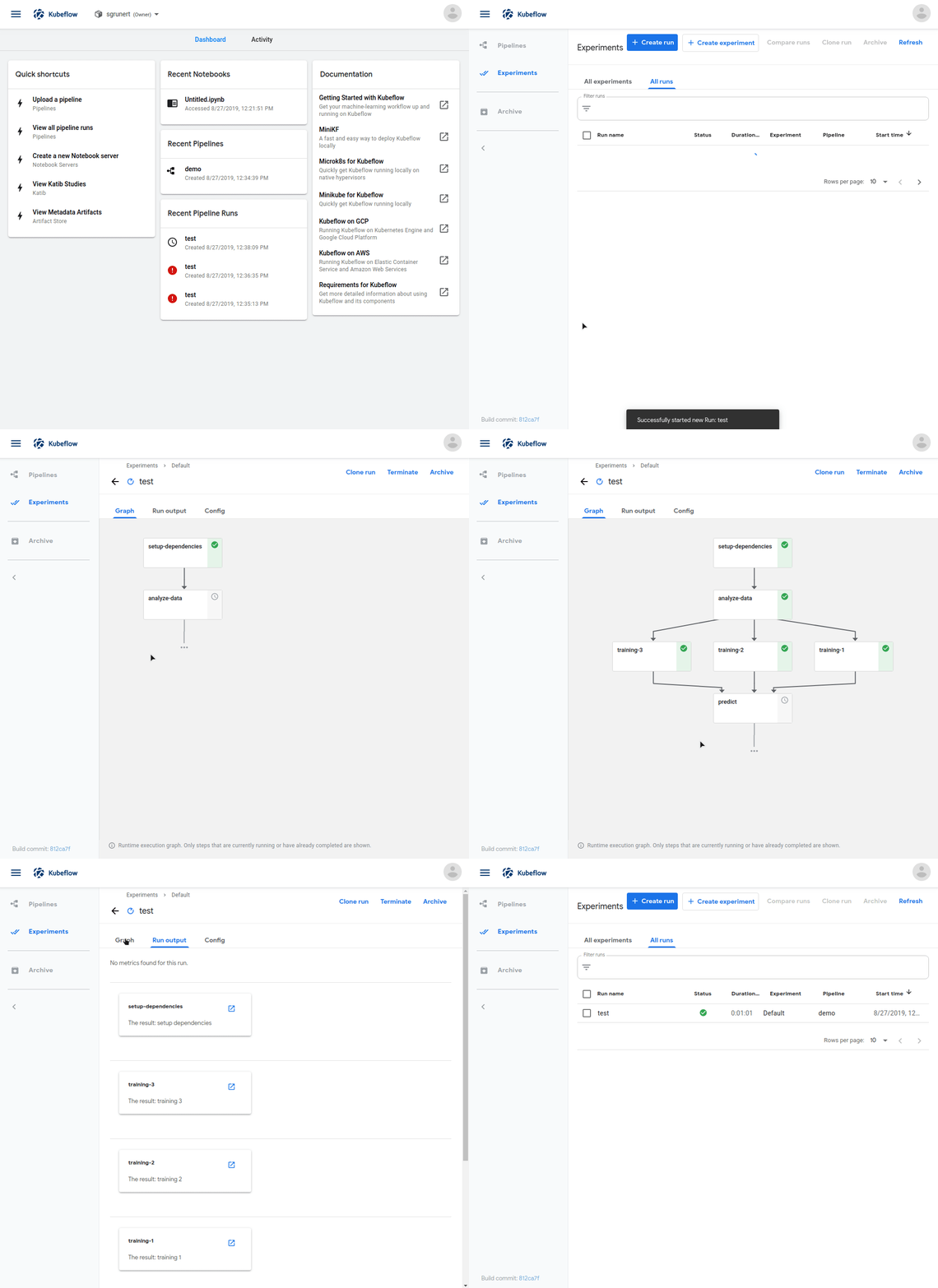
How could such a pipeline look like? For the first scenario, we created a pseudo pipeline called demo. This pipeline can be executed in so-called experiments, which looks like this:

Every pipeline step is executed directly in Kubernetes within its own pod, whereas inputs and outputs for each step can be passed around too. Kubeflow is also able to display graphics like receiver operating characteristic (ROC) charts or confusion matrices. All in all, a single trivial pipeline step would look like this Python snippet:

from kfp.dsl import ContainerOp

step1 = ContainerOp(name='step1',
                    image='alpine:latest',
                    command=['sh', '-c'],
                    arguments=['echo "Running step"'])

This step would do nothing else than echoing "Running step". To bring multiple steps into dependency with each other, we could create a second step2 and run:

step2.after(step1)

A complete pipeline example would look like this, where we have to outline it with @pipeline and compile it afterwards via compile():

from kfp.compiler import Compiler
from kfp.dsl import ContainerOp, pipeline


@pipeline(name='My pipeline', description='')
def pipeline():
    step1 = ContainerOp(name='step1',
                        image='alpine:latest',
                        command=['sh', '-c'],
                        arguments=['echo "Running step"'])
    step2 = ContainerOp(name='step2',
                        image='alpine:latest',
                        command=['sh', '-c'],
                        arguments=['echo "Running step"'])
    step2.after(step1)


if __name__ == '__main__':
    Compiler().compile(pipeline)

This kind of pipeline component can especially be useful for deployment tasks, or even querying for new data. The downside of this approach is the need for an executable to be run. Typical data science tasks, like training a model would require a dedicated training script to be available as part of the base image.

This approach may get a little impractical considering the fact that data science tasks quite often consist of short one-line code snippets. Due to that, Kubeflow offers the possibility to create lightweight components from Python directly. Such a component may look like this:

from kfp.components import func_to_container_op

def sum_sq(a: int, b: int) -> int:
    import numpy
    dist = np.sqrt(a**2 + b**2)
    return dist

add_op = func_to_container_op(sum_sq)(1, 2)

Running this pipeline would deliver the inputs sum of squares as the pipelines output. Even though, this approach can really reduce the afford to describe a component, but there are a few restrictions to be considered:

• Lightweight functions need to be standalone, so they may not use code, imports or variables defined in another scope.
• Imported packages needs to be available in the container image.
• Input parameters needs to be set to str (default), int or float which are the only types currently supported (Google Cloud Platform provides methods to overcome this limitation)

This is due to the fact, that the Kubeflow will internally create an executable command similar to:

python -u -c "def sum_sq(a: int, b:int):\n\
                import numpy\n\
                dist = np.sqrt(a**2 + b**2)\n\
                return dist\n(...)"

Respecting all these limitations, a lightweight component for training a model may look like this:

from kfp.components import func_to_container_op


def fit_squeezenet(pretrained: bool = False):
    from fastai.vision import cnn_learner, accuracy, models
    name: str = "squeezenet.model"
    loader = ImageDataBunch.from_folder("test/images",
                                        train="training",
                                        valid="test",
                                        size=112)
    learner = cnn_learner(loader,
                          models.squeezenet1_0,
                          pretrained=pretrained,
                          metrics=accuracy,
                          silent=False,
                          add_time=True)

    learner.fit_one_cycle(1)

We could also split up components by saving and loading output from or to a persistent volume. Our pipeline would then look somewhat like this:

from kfp.components import func_to_container_op


def fit_squeezenet(loader: str,
                   storage: str,
                   pretrained: bool = False,
                   name: str = "squeezenet.model") -> str:
    import dill
    from fastai.vision import cnn_learner, accuracy, models
    import codecs

    with open(outpath, "rb") as fp:
        learner = dill.load(fp)

    loader = dill.loads(codecs.decode(loader.encode(), "base64"))
    learner = cnn_learner(loader,
                          models.squeezenet1_0,
                          pretrained=False,
                          metrics=accuracy,
                          silent=False,
                          add_time=True)
    learner.fit_one_cycle(1)

    outpath = storage + "/" + name
    with open(outpath, "wb") as fp:
        dill.dump(learner, fp)

    return outpath


op = func_to_container_op(fit_squeezenet,
                          base_image="alpine:latest")("out/model", False,
                                                      "squeeze.model")
op.add_volume(
    k8s.V1Volume(name='volume',
                 host_path=k8s.V1HostPathVolumeSource(
                     path='/data/out'))).add_volume_mount(
                         k8s.V1VolumeMount(name='volume', mount_path="out"))

For even complexer scenarios, creating a dedicated training script and executing it within a ContainerOp directly as shown above may be the best best. Now that we know how to properly describe a pipeline let’s see how to run one.

We have to compile the pipeline via the dsl-compile executable from the pipelines SDK:

> sudo pip install https://storage.googleapis.com/ml-pipeline/release/0.1.27/kfp.tar.gz
> dsl-compile --py pipeline.py --output pipeline.tar.gz

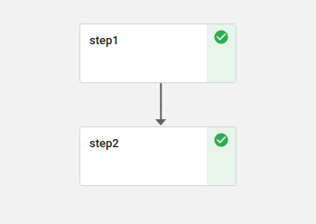
The resulting tarball can now be uploaded to Kubeflow via the web dashboard and executed there. If the pipeline run is done, then the graph should look like this:

All pipelines are internally transformed to Argo workflows which are part of the Argo CD application Kubeflow uses for its execution. With the help of the Argo CLI we can examine the pipeline even further:

> kubectl get workflow
NAME                AGE
my-pipeline-8lwcc   6m47s

> argo get my-pipeline-8lwcc
Name:                my-pipeline-8lwcc
Namespace:           kubeflow
ServiceAccount:      pipeline-runner
Status:              Succeeded
Created:             Tue Aug 27 13:06:06 +0200 (4 minutes ago)
Started:             Tue Aug 27 13:06:06 +0200 (4 minutes ago)
Finished:            Tue Aug 27 13:06:22 +0200 (4 minutes ago)
Duration:            16 seconds

STEP                  PODNAME                      DURATION  MESSAGE
 ✔ my-pipeline-8lwcc
 ├-✔ step1            my-pipeline-8lwcc-818794353  6s
 └-✔ step2            my-pipeline-8lwcc-768461496  7s

This should give us a good feeling about how Kubeflow uses third party software to actually do the job.

Please note that we had to modify the pipelines to work on Kubernetes deployments which are not running Docker as container runtime under the hood. The full working examples can be found in 0-demo.py and 1-demo.py.

Machine Learning Pipelines within Notebooks

Jupyter notebooks are a very common choice for building and evaluating machine learning models. As they can be run within Kubeflow with barely one click, wouldn’t it be nice to additionally be in control over the pipeline system from there as well? Luckily Kubeflow got your back!

By importing the kfp.compiler package into a notebook the previous pipeline steps can be done from a notebook directly. This also empowers us to create experiments and pipeline runs in an integrated manner from within Jupyter. Let’s say we have created a pipeline called training_pipeline. Then we would import the kfp compiler and build the pipeline like this:

from kfp.compiler import Compiler
pipeline_func = training_pipeline
pipeline_filename = pipeline_func.__name__ + '.pipeline.yaml'
Compiler().compile(pipeline_func, pipeline_filename)

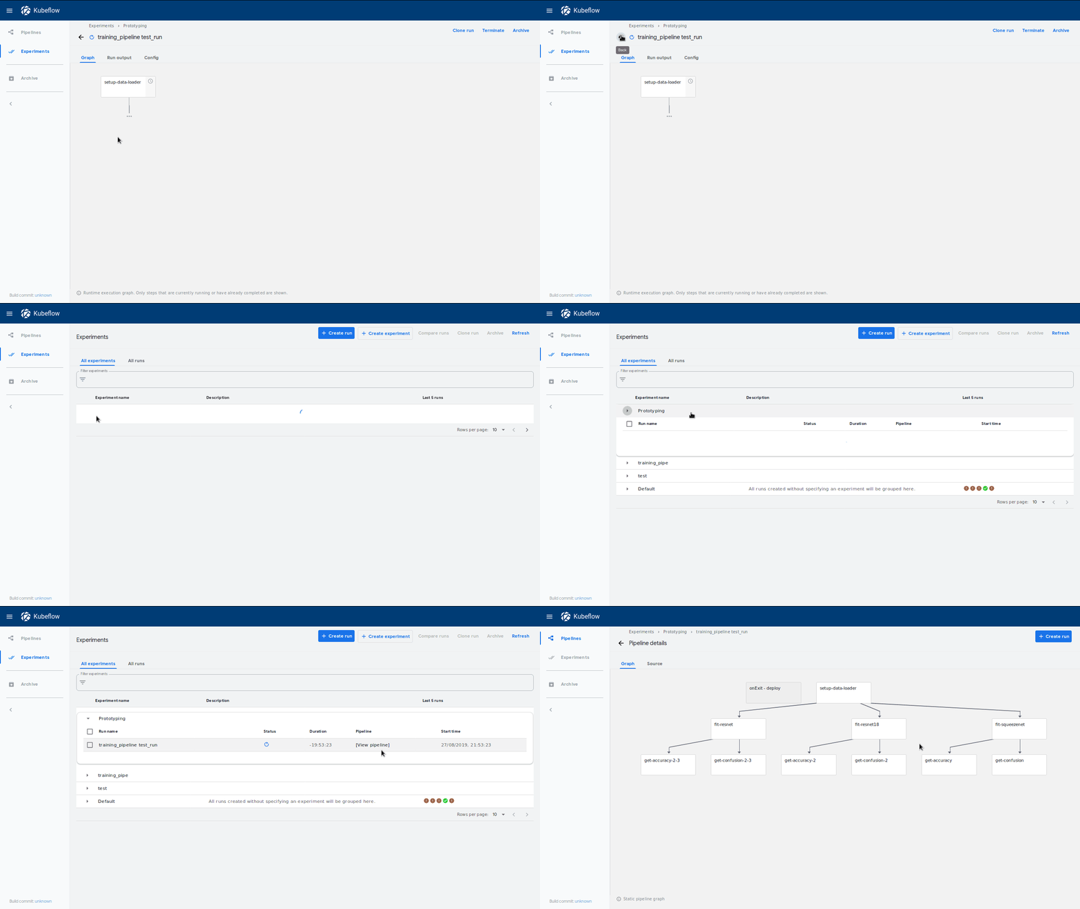
This will put the pipeline definition to a YAML file and enable us to upload this file to our pipeline endpoint. To do so let’s first of all create a new experiment:

import kfp
client = kfp.Client()

try:
    experiment = client.create_experiment("Prototyping")
except Exception:
    experiment = client.get_experiment(experiment_name="Prototyping")

Afterwards we can trigger a run directly from the Jupyter notebook:

arguments = {'pretrained': 'False'}
run_name = pipeline_func.__name__ + ' test_run'
run_result = client.run_pipeline(experiment.id, run_name, pipeline_filename, arguments)

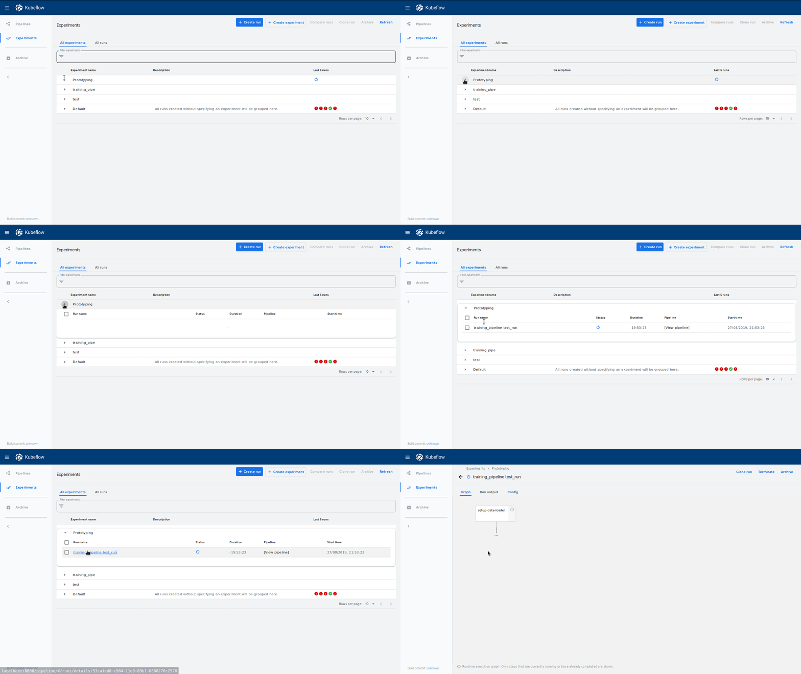
This will create a new run called training_pipeline test_run within an experiment called Prototype. A neat feature is that a link to this experiment will be shown immediately, which will lead to our dashboard where our run has started:

We can also check if the pipeline structure is the expected one by clicking on View Pipeline.

Neat! We have successfully deployed a pipeline from our notebook. There are a few things that significantly can be seen as improvements to the classical workflow. First of all, we have set up a reproducible way of handling our model. If the pipeline fits our needs we could simply deploy it as a recurring run and our model would stay up-to-date on a regular basis. On the other hand, we could also use the pipeline system within the prototyping process to unblock us from waiting for single steps in the notebook to be finished.

Continuous Integration Lookout

All our steps we did so far were more or less driven by manual intervention. But to fully unleash the power of an automated CI/CD process, we would need to somehow automate our workflow completely.

Luckily, Kubeflow provides a pipelines REST API which can be used for such tasks. For demonstration purposes we now bypass the required authentication via kube-proxy by executing:

> kubectl port-forward -n kubeflow svc/ml-pipeline 8888
Forwarding from 127.0.0.1:8888 -> 8888
Forwarding from [::1]:8888 -> 8888

The API serves now on localhost:8888, where we’re able to upload our demo project from the command line:

> dsl-compile --py 0-demo.py --output demo-0.tar.gz
> curl -F [email protected] http://localhost:8888/apis/v1beta1/pipelines/upload\?name=demo-0
{"id":"09f6113b-1646-4333-ba97-3008c046b5a6","name":"demo-0","created_at":"2019-08-30T09:10:45Z"}

A new run can now be started by utilizing the runs API and passing in the correct pipeline_id, which is 09f6113b-1646-4333-ba97-3008c046b5a6 in our case:

> curl http://localhost:8888/apis/v1beta1/runs -H 'Content-Type: application/json' \
        --data-binary '{
            "name":"my-run",
            "pipeline_spec": {
                "pipeline_id":"09f6113b-1646-4333-ba97-3008c046b5a6"
            }
        }' | jq .run.id
"0ee04b48-69c0-40e3-b286-683957fcc283"

We’re now able to track the results from the run by polling the API:

> curl http://localhost:8888/apis/v1beta1/runs/0ee04b48-69c0-40e3-b286-683957fcc283 | jq .run.status
"Succeeded"

Pretty great, a possible fully automated CI/CD workflow could now build the pipeline via dsl-compile, push it into a new test experiment and create the runs. If the run succeeds, then we could update the served model internally. Kubeflow wouldn’t be Kubeflow if there would be no solution for that: Serving TensorFlow or PyTorch based models is possible via Kubeflow too!

Covering this topic as well would go beyond of the scope of this blog post so we will leave this open to your personal discovery session with Kubeflow.

Conclusion

So, that’s it for now. We hope you enjoyed the read getting a feeling about cloud native applications and Kubeflow. We think that Kubeflow has a bright future and would like to encourage you to contribute to the project to support the maintainers.