SciPyDiffEq.jl

![]()
SciPyDiffEq.jl is a common interface binding for the SciPy solve_ivp module ordinary differential equation solvers. It uses the PyCall.jl interop in order to send the differential equation over to Python and solve it.
Note that this package isn't for production use and is mostly just for benchmarking and helping new users migrate models over to Julia. For more efficient solvers, see the DifferentialEquations.jl documentation.
Installation
To install SciPyDiffEq.jl, use the following:
Pkg.clone("https://github.com/JuliaDiffEq/SciPyDiffEq.jl")Using SciPyDiffEq.jl
SciPyDiffEq.jl is simply a solver on the DiffEq common interface, so for details see the DifferentialEquations.jl documentation. The available algorithms are:
SciPyDiffEq.RK45
SciPyDiffEq.RK23
SciPyDiffEq.Radau
SciPyDiffEq.BDF
SciPyDiffEq.LSODA
SciPyDiffEq.odeint
Example
using SciPyDiffEq

function lorenz(u,p,t)
 du1 = 10.0(u[2]-u[1])
 du2 = u[1]*(28.0-u[3]) - u[2]
 du3 = u[1]*u[2] - (8/3)*u[3]
 [du1, du2, du3]
end
tspan = (0.0,10.0)
u0 = [1.0,0.0,0.0]
prob = ODEProblem(lorenz,u0,tspan)
sol = solve(prob,SciPyDiffEq.RK45())
Measuring Overhead
In the following we can measure the overhead and show that using SciPy from Julia is about 3x faster than using SciPy with Numba. Using SciPyDiffEq:
using SciPyDiffEq, BenchmarkTools

function lorenz(u,p,t)
    du1 = 10.0(u[2]-u[1])
    du2 = u[1]*(28.0-u[3]) - u[2]
    du3 = u[1]*u[2] - (8/3)*u[3]
    [du1, du2, du3]
end
tspan = (0.0,100.0)
u0 = [1.0,0.0,0.0]
prob = ODEProblem(lorenz,u0,tspan)
@btime sol = solve(prob,SciPyDiffEq.RK45(),dense=false, abstol=1e-8,reltol=1e-8) # 2.760 s (4426860 allocations: 182.27 MiB)
This gives 2.76s. Solving the equivalent problem with SciPy odeint is:
import numpy as np
from scipy.integrate import odeint
import timeit
import numba
def f(u, t):
    x, y, z = u
    return [10.0 * (y - x), x * (28.0 - z) - y, x * y - 2.66 * z]

u0 = [1.0,0.0,0.0]
tspan = (0., 100.)
t = np.linspace(0, 100, 1001)
sol = odeint(f, u0, t)
def time_func():
    odeint(f, u0, t, rtol = 1e-8, atol=1e-8)

_t = timeit.Timer(time_func).timeit(number=100)
print(_t) # 13.898981100000015 seconds
which takes 13.89 seconds. Then using Numba JIT with nopython mode is:
numba_f = numba.jit(f,nopython=True)
odeint(numba_f, u0, t,rtol = 1e-8, atol=1e-8)

def time_func():
   odeint(numba_f, u0, t,rtol = 1e-8, atol=1e-8)

_t = timeit.Timer(time_func).timeit(number=100)
print(_t) # 8.05035870000006 seconds
which takes 8 seconds. Solving it with SciPy solve_ivp is:
import numpy as np
from scipy.integrate import solve_ivp
import timeit
import numba
def f(t,u):
    x, y, z = u
    return [10.0 * (y - x), x * (28.0 - z) - y, x * y - 2.66 * z]

u0 = [1.0,0.0,0.0]
tspan = (0.0, 100.0)
t = np.linspace(0, 100, 1001)
sol = solve_ivp(f,(0.0, 100.0),u0,t_eval=t)

def time_func():
    solve_ivp(f,(0.0, 100.0),u0,t_eval=t)

_t = timeit.Timer(time_func).timeit(number=100)
print(_t) # 15.978812399999999 seconds
and
numba_f = numba.jit(f,nopython=True)
sol = solve_ivp(numba_f,(0.0, 100.0),u0,t_eval=t)

def time_func():
   solve_ivp(numba_f,(0.0, 100.0),u0,t_eval=t)

_t = timeit.Timer(time_func).timeit(number=100)
print(_t) # 14.302745000000002 seconds
which Numba seems to be unable to effectively accelerate. Together, this
showcases a 3x speedup over the best SciPy+Numba setup by using the Julia based
interface, (and 5x head-to-head via solve_ivp) so overhead concerns in future
benchmarks are gone because any measurement here is accelerating SciPy more
than standard accelerated use.
Benchmarks
The following benchmarks demonstrate a 50x-1,000x performance advantage for the pure-Julia methods over the Julia-accelerated (3x) SciPy ODE solvers across a range of stiff and non-stiff ODEs. These were ran with Julia 1.2, MATLAB 2019B, deSolve 1.2.5, and SciPy 1.3.1 after verifying negligible overhead on interop.
Non-Stiff Problem 1: Lotka-Volterra
f = @ode_def_bare LotkaVolterra begin
  dx = a*x - b*x*y
  dy = -c*y + d*x*y
end a b c d
p = [1.5,1,3,1]
tspan = (0.0,10.0)
u0 = [1.0,1.0]
prob = ODEProblem(f,u0,tspan,p)
sol = solve(prob,Vern7(),abstol=1/10^14,reltol=1/10^14)
test_sol = TestSolution(sol)

setups = [Dict(:alg=>DP5())
          Dict(:alg=>dopri5())
          Dict(:alg=>Tsit5())
          Dict(:alg=>Vern7())
          Dict(:alg=>MATLABDiffEq.ode45())
          Dict(:alg=>MATLABDiffEq.ode113())
          Dict(:alg=>SciPyDiffEq.RK45())
          Dict(:alg=>SciPyDiffEq.LSODA())
          Dict(:alg=>SciPyDiffEq.odeint())
          Dict(:alg=>deSolveDiffEq.lsoda())
          Dict(:alg=>deSolveDiffEq.ode45())
          Dict(:alg=>CVODE_Adams())
  ]

names = [
  "Julia: DP5"
  "Hairer: dopri5"
  "Julia: Tsit5"
  "Julia: Vern7"
  "MATLAB: ode45"
  "MATLAB: ode113"
  "SciPy: RK45"
  "SciPy: LSODA"
  "SciPy: odeint"
  "deSolve: lsoda"
  "deSolve: ode45"
  "Sundials: Adams"
  ]

abstols = 1.0 ./ 10.0 .^ (6:13)
reltols = 1.0 ./ 10.0 .^ (3:10)
wp = WorkPrecisionSet(prob,abstols,reltols,setups;
                      names = names,
                      appxsol=test_sol,dense=false,
                      save_everystep=false,numruns=100,maxiters=10000000,
                      timeseries_errors=false,verbose=false)
plot(wp,title="Non-stiff 1: Lotka-Volterra")
Non-Stiff Problem 2: Rigid Body
f = @ode_def_bare RigidBodyBench begin
  dy1  = -2*y2*y3
  dy2  = 1.25*y1*y3
  dy3  = -0.5*y1*y2 + 0.25*sin(t)^2
end
prob = ODEProblem(f,[1.0;0.0;0.9],(0.0,100.0))
sol = solve(prob,Vern7(),abstol=1/10^14,reltol=1/10^14)
test_sol = TestSolution(sol)

setups = [Dict(:alg=>DP5())
          Dict(:alg=>dopri5())
          Dict(:alg=>Tsit5())
          Dict(:alg=>Vern7())
          Dict(:alg=>MATLABDiffEq.ode45())
          Dict(:alg=>MATLABDiffEq.ode113())
          Dict(:alg=>SciPyDiffEq.RK45())
          Dict(:alg=>SciPyDiffEq.LSODA())
          Dict(:alg=>SciPyDiffEq.odeint())
          Dict(:alg=>deSolveDiffEq.lsoda())
          Dict(:alg=>deSolveDiffEq.ode45())
          Dict(:alg=>CVODE_Adams())
  ]

names = [
  "Julia: DP5"
  "Hairer: dopri5"
  "Julia: Tsit5"
  "Julia: Vern7"
  "MATLAB: ode45"
  "MATLAB: ode113"
  "SciPy: RK45"
  "SciPy: LSODA"
  "SciPy: odeint"
  "deSolve: lsoda"
  "deSolve: ode45"
  "Sundials: Adams"
  ]

abstols = 1.0 ./ 10.0 .^ (6:13)
reltols = 1.0 ./ 10.0 .^ (3:10)
wp = WorkPrecisionSet(prob,abstols,reltols,setups;
                      names = names,
                      appxsol=test_sol,dense=false,
                      save_everystep=false,numruns=100,maxiters=10000000,
                      timeseries_errors=false,verbose=false)
plot(wp,title="Non-stiff 2: Rigid-Body")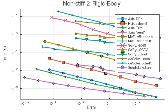
Stiff Problem 1: ROBER
rober = @ode_def begin
  dy₁ = -k₁*y₁+k₃*y₂*y₃
  dy₂ =  k₁*y₁-k₂*y₂^2-k₃*y₂*y₃
  dy₃ =  k₂*y₂^2
end k₁ k₂ k₃
prob = ODEProblem(rober,[1.0,0.0,0.0],(0.0,1e5),[0.04,3e7,1e4])
sol = solve(prob,CVODE_BDF(),abstol=1/10^14,reltol=1/10^14)
test_sol = TestSolution(sol)

abstols = 1.0 ./ 10.0 .^ (7:8)
reltols = 1.0 ./ 10.0 .^ (3:4);

setups = [Dict(:alg=>Rosenbrock23())
          Dict(:alg=>TRBDF2())
          Dict(:alg=>RadauIIA5())
          Dict(:alg=>rodas())
          Dict(:alg=>radau())
          Dict(:alg=>MATLABDiffEq.ode23s())
          Dict(:alg=>MATLABDiffEq.ode15s())
          Dict(:alg=>SciPyDiffEq.LSODA())
          Dict(:alg=>SciPyDiffEq.BDF())
          Dict(:alg=>SciPyDiffEq.odeint())
          Dict(:alg=>deSolveDiffEq.lsoda())
          Dict(:alg=>CVODE_BDF())
          ]

names = [
  "Julia: Rosenbrock23"
  "Julia: TRBDF2"
  "Julia: radau"
  "Hairer: rodas"
  "Hairer: radau"
  "MATLAB: ode23s"
  "MATLAB: ode15s"
  "SciPy: LSODA"
  "SciPy: BDF"
  "SciPy: odeint"
  "deSolve: lsoda"
  "Sundials: CVODE"
  ]

wp = WorkPrecisionSet(prob,abstols,reltols,setups;
                      names = names,print_names = true,
                      dense=false,verbose = false,
                      save_everystep=false,appxsol=test_sol,
                      maxiters=Int(1e5))
plot(wp,title="Stiff 1: ROBER", legend=:topleft)
Stiff Problem 2: HIRES
f = @ode_def Hires begin
  dy1 = -1.71*y1 + 0.43*y2 + 8.32*y3 + 0.0007
  dy2 = 1.71*y1 - 8.75*y2
  dy3 = -10.03*y3 + 0.43*y4 + 0.035*y5
  dy4 = 8.32*y2 + 1.71*y3 - 1.12*y4
  dy5 = -1.745*y5 + 0.43*y6 + 0.43*y7
  dy6 = -280.0*y6*y8 + 0.69*y4 + 1.71*y5 -
           0.43*y6 + 0.69*y7
  dy7 = 280.0*y6*y8 - 1.81*y7
  dy8 = -280.0*y6*y8 + 1.81*y7
end

u0 = zeros(8)
u0[1] = 1
u0[8] = 0.0057
prob = ODEProblem(f,u0,(0.0,321.8122))

sol = solve(prob,Rodas5(),abstol=1/10^14,reltol=1/10^14)
test_sol = TestSolution(sol)

abstols = 1.0 ./ 10.0 .^ (5:8)
reltols = 1.0 ./ 10.0 .^ (1:4);

setups = [Dict(:alg=>Rosenbrock23())
          Dict(:alg=>TRBDF2())
          Dict(:alg=>RadauIIA5())
          Dict(:alg=>rodas())
          Dict(:alg=>radau())
          Dict(:alg=>MATLABDiffEq.ode23s())
          Dict(:alg=>MATLABDiffEq.ode15s())
          Dict(:alg=>SciPyDiffEq.LSODA())
          Dict(:alg=>SciPyDiffEq.BDF())
          Dict(:alg=>SciPyDiffEq.odeint())
          Dict(:alg=>deSolveDiffEq.lsoda())
          Dict(:alg=>CVODE_BDF())
          ]

names = [
  "Julia: Rosenbrock23"
  "Julia: TRBDF2"
  "Julia: radau"
  "Hairer: rodas"
  "Hairer: radau"
  "MATLAB: ode23s"
  "MATLAB: ode15s"
  "SciPy: LSODA"
  "SciPy: BDF"
  "SciPy: odeint"
  "deSolve: lsoda"
  "Sundials: CVODE"
  ]

wp = WorkPrecisionSet(prob,abstols,reltols,setups;
                      names = names,print_names = true,
                      save_everystep=false,appxsol=test_sol,
                      maxiters=Int(1e5),numruns=100)
plot(wp,title="Stiff 2: Hires",legend=:topleft)