Stheno

Stheno is an implementation of Gaussian process modelling in Python. See also Stheno.jl.

• Nonlinear Regression in 20 Seconds
• Installation
• Manual
  • AutoGrad, TensorFlow, PyTorch, or Jax? Your Choice!
  • Important Remarks
  • Model Design
  • Finite-Dimensional Distributions
  • Prior and Posterior Measures
  • Inducing Points
  • Mean and Kernel Design
• Examples
  • Simple Regression
  • Decomposition of Prediction
  • Learn a Function, Incorporating Prior Knowledge About Its Form
  • Multi-Output Regression
  • Approximate Integration
  • Bayesian Linear Regression
  • GPAR
  • A GP-RNN Model
  • Approximate Multiplication Between GPs
  • Sparse Regression
  • Smoothing with Nonparametric Basis Functions

Nonlinear Regression in 20 Seconds

>>> import numpy as np

>>> from stheno import Measure, GP, EQ

>>> x = np.linspace(0, 2, 10)          # Some points to predict at

>>> y = x ** 2                         # Some observations

>>> prior = Measure()                  # Construct a prior.

>>> f = GP(EQ(), measure=prior)        # Define our probabilistic model.

>>> post = prior | (f(x), y)           # Compute the posterior distribution.

>>> post(f).mean(np.array([1, 2, 3]))  # Predict!
<dense matrix: shape=3x1, dtype=float64
 mat=[[1.   ]
      [4.   ]
      [8.483]]>

Moar?! Then read on!

Installation

See the instructions here. Then simply

pip install stheno

Manual

Note: here is a nicely rendered and more readable version of the docs.

AutoGrad, TensorFlow, PyTorch, or Jax? Your Choice!

from stheno.autograd import GP, EQ

from stheno.tensorflow import GP, EQ

from stheno.torch import GP, EQ

from stheno.jax import GP, EQ

Important Remarks

Stheno uses LAB to provide an implementation that is backend agnostic. Moreover, Stheno uses an extension of LAB to accelerate linear algebra with structured linear algebra primitives. You will encounter these primitives:

>>> k = 2 * Delta()

>>> x = np.linspace(0, 5, 10)

>>> k(x)
<diagonal matrix: shape=10x10, dtype=float64
 diag=[2. 2. 2. 2. 2. 2. 2. 2. 2. 2.]>

If you're using LAB to further process these matrices, then there is absolutely no need to worry: these structured matrix types know how to add, multiply, and do other linear algebra operations.

>>> import lab as B

>>> B.matmul(k(x), k(x))
<diagonal matrix: shape=10x10, dtype=float64
 diag=[4. 4. 4. 4. 4. 4. 4. 4. 4. 4.]>

If you're not using LAB, you can convert these structured primitives to regular NumPy/TensorFlow/PyTorch/Jax arrays by calling B.dense (B is from LAB):

>>> import lab as B

>>> B.dense(k(x))
array([[2., 0., 0., 0., 0., 0., 0., 0., 0., 0.],
       [0., 2., 0., 0., 0., 0., 0., 0., 0., 0.],
       [0., 0., 2., 0., 0., 0., 0., 0., 0., 0.],
       [0., 0., 0., 2., 0., 0., 0., 0., 0., 0.],
       [0., 0., 0., 0., 2., 0., 0., 0., 0., 0.],
       [0., 0., 0., 0., 0., 2., 0., 0., 0., 0.],
       [0., 0., 0., 0., 0., 0., 2., 0., 0., 0.],
       [0., 0., 0., 0., 0., 0., 0., 2., 0., 0.],
       [0., 0., 0., 0., 0., 0., 0., 0., 2., 0.],
       [0., 0., 0., 0., 0., 0., 0., 0., 0., 2.]])

Furthermore, before computing a Cholesky decomposition, Stheno always adds a minuscule diagonal to prevent the Cholesky decomposition from failing due to positive indefiniteness caused by numerical noise. You can change the magnitude of this diagonal by changing B.epsilon:

>>> import lab as B

>>> B.epsilon = 1e-12   # Default regularisation

>>> B.epsilon = 1e-8    # Strong regularisation

Model Design

The basic building block is a f = GP(mean=0, kernel, measure=prior), which takes in a mean, a kernel, and a measure. The mean and kernel of a GP can be extracted with f.mean and f.kernel. The measure should be thought of as a big joint distribution that assigns a mean and a kernel to every variable f. A measure can be created with prior = Measure(). A GP f can have different means and kernels under different measures. For example, under some prior measure, f can have an EQ() kernel; but, under some posterior measure, f has a kernel that is determined by the posterior distribution of a GP. We will see later how posterior measures can be constructed. The measure with which a f = GP(kernel, measure=prior) is constructed can be extracted with f.measure == prior. If the keyword argument measure is not set, then automatically a new measure is created, which afterwards can be extracted with f.measure.

Definition, where prior = Measure():

f = GP(kernel)

f = GP(mean, kernel)

f = GP(kernel, measure=prior)

f = GP(mean, kernel, measure=prior)

GPs that are associated to the same measure can be combined into new GPs, which is the primary mechanism used to build cool models.

Here's an example model:

>>> prior = Measure()

>>> f1 = GP(lambda x: x ** 2, EQ(), measure=prior)

>>> f1
GP(<lambda>, EQ())

>>> f2 = GP(Linear(), measure=prior)

>>> f2
GP(0, Linear())

>>> f_sum = f1 + f2

>>> f_sum
GP(<lambda>, EQ() + Linear())

>>> f_sum + GP(EQ())  # Not valid: `GP(EQ())` belongs to a new measure!
AssertionError: Processes GP(<lambda>, EQ() + Linear()) and GP(0, EQ()) are associated to different measures.

Compositional Design

• Add and subtract GPs and other objects.

  Example:

  >>> GP(EQ(), measure=prior) + GP(Exp(), measure=prior)
  GP(0, EQ() + Exp())
  
  >>> GP(EQ(), measure=prior) + GP(EQ(), measure=prior)
  GP(0, 2 * EQ())
  
  >>> GP(EQ()) + 1
  GP(1, EQ())
  
  >>> GP(EQ()) + 0
  GP(0, EQ())
  
  >>> GP(EQ()) + (lambda x: x ** 2)
  GP(<lambda>, EQ())
  
  >>> GP(2, EQ(), measure=prior) - GP(1, EQ(), measure=prior)
  GP(1, 2 * EQ())
  

• Add and subtract GPs and other objects.

  Warning: The product of two GPs it not a Gaussian process. Stheno approximates the resulting process by moment matching.

  Example:

  >>> GP(1, EQ(), measure=prior) * GP(1, Exp(), measure=prior)
  GP(<lambda> + <lambda> + -1 * 1, <lambda> * Exp() + <lambda> * EQ() + EQ() * Exp())
  
  >>> 2 * GP(EQ())
  GP(2, 2 * EQ())
  
  >>> 0 * GP(EQ())
  GP(0, 0)
  
  >>> (lambda x: x) * GP(EQ())
  GP(0, <lambda> * EQ())
  

• Shift GPs.

  Example:

  >>> GP(EQ()).shift(1)
  GP(0, EQ() shift 1) 
  

• Stretch GPs.

  Example:

  >>> GP(EQ()).stretch(2)
  GP(0, EQ() > 2)
  

  The > operator is implemented to provide a shorthand for stretching:

  >>> GP(EQ()) > 2
  GP(0, EQ() > 2)
  

• Select particular input dimensions.

  Example:

  >>> GP(EQ()).select(1, 3)
  GP(0, EQ() : [1, 3])
  

  Indexing is implemented to provide a a shorthand for selecting input dimensions:

  >>> GP(EQ())[1, 3]
  GP(0, EQ() : [1, 3]) 
  

• Transform the input.

  Example:

  >>> GP(EQ()).transform(f)
  GP(0, EQ() transform f)
  

• Numerically take the derivative of a GP. The argument specifies which dimension to take the derivative with respect to.

  Example:

  >>> GP(EQ()).diff(1)
  GP(0, d(1) EQ())
  

• Construct a finite difference estimate of the derivative of a GP. See stheno.measure.Measure.diff_approx for a description of the arguments.

  Example:

  >>> GP(EQ()).diff_approx(deriv=1, order=2)
  GP(50000000.0 * (0.5 * EQ() + 0.5 * ((-0.5 * (EQ() shift (0.0001414213562373095, 0))) shift (0, -0.0001414213562373095)) + 0.5 * ((-0.5 * (EQ() shift (0, 0.0001414213562373095))) shift (-0.0001414213562373095, 0))), 0)
  

• Construct the Cartesian product of a collection of GPs.

  Example:

  >>> prior = Measure()
  
  >>> f1, f2 = GP(EQ(), measure=prior), GP(EQ(), measure=prior)
  
  >>> cross(f1, f2)
  GP(MultiOutputMean(0, 0), MultiOutputKernel(EQ(), EQ()))
  

Displaying GPs

Like means and kernels, GPs have a display method that accepts a formatter.

Example:

>>> print(GP(2.12345 * EQ()).display(lambda x: '{:.2f}'.format(x)))
GP(2.12 * EQ(), 0)

Properties of GPs

Properties of kernels can be queried on GPs directly.

Example:

>>> GP(EQ()).stationary
True

Naming GPs

It is possible to give a name to a GP. Names must be strings. A measure then behaves like a two-way dictionary between GPs and their names.

Example:

>>> prior = Measure()

>>> p = GP(EQ(), name='name', measure=prior)

>>> p.name
'name'

>>> p.name = 'alternative_name'

>>> prior['alternative_name']
GP(0, EQ())

>>> prior[p]
'alternative_name'

Finite-Dimensional Distributions

Simply call a GP to construct a finite-dimensional distribution. You can then compute the mean, the variance, sample, or compute a logpdf.

Example:

>>> prior = Measure()

>>> f = GP(EQ(), measure=prior)

>>> x = np.array([0., 1., 2.])

>>> f(x)
FDD(GP(0, EQ()), array([0., 1., 2.]))

>>> f(x).mean
array([[0.],
       [0.],
       [0.]])

>>> f(x).var
<dense matrix: shape=3x3, dtype=float64
 mat=[[1.    0.607 0.135]
      [0.607 1.    0.607]
      [0.135 0.607 1.   ]]>
       
>>> y1 = f(x).sample()

>>> y1
array([[-0.45172746],
       [ 0.46581948],
       [ 0.78929767]])
       
>>> f(x).logpdf(y1)
-2.811609567720761

>>> y2 = f(x).sample(2)
array([[-0.43771276, -2.36741858],
       [ 0.86080043, -1.22503079],
       [ 2.15779126, -0.75319405]]

>>> f(x).logpdf(y2)
 array([-4.82949038, -5.40084225])

• Use f(x).marginals() to efficiently compute the means and the marginal lower and upper 95% central credible region bounds.

  Example:

  >>> f(x).marginals()
  (array([0., 0., 0.]), array([-1.96, -1.96, -1.96]), array([1.96, 1.96, 1.96]))
  

• Use Measure.logpdf to compute the joint logpdf of multiple observations.

  Definition:

  prior.logpdf(f(x), y)
  
  prior.logpdf((f1(x1), y1), (f2(x2), y2), ...)
  

• Use Measure.sample to jointly sample multiple observations.

  Definition, where prior = Measure():

  sample = prior.sample(f(x))
  
  sample1, sample2, ... = prior.sample(f1(x1), f2(x2), ...)
  

Prior and Posterior Measures

Conditioning a prior measure on observations gives a posterior measure. To condition a measure on observations, use Measure.__or__.

Definition, where prior = Measure() and f* and g* are GPs:

post = prior | (f(x), y)

post = prior | ((f1(x1), y1), (f2(x2), y2), ...)

You can then obtain a posterior process with post(f) and a finite-dimensional distribution under the posterior with post(f(x)).

Let's consider an example. First, build a model and sample some values.

>>> prior = Measure()

>>> f = GP(EQ(), measure=prior)

>>> x = np.array([0., 1., 2.])

>>> y = f(x).sample()

Then compute the posterior measure.

>>> post = prior | (f(x), y)

>>> post(f)
GP(PosteriorMean(), PosteriorKernel())

>>> post(f).mean(x)
<dense matrix: shape=3x1, dtype=float64
 mat=[[ 0.412]
      [-0.811]
      [-0.933]]>

>>> post(f).kernel(x)
<dense matrix: shape=3x3, dtype=float64
 mat=[[1.e-12 0.e+00 0.e+00]
      [0.e+00 1.e-12 0.e+00]
      [0.e+00 0.e+00 1.e-12]]>

>>> post(f(x))
<stheno.random.Normal at 0x7fa6d7f8c358>

>>> post(f(x)).mean
<dense matrix: shape=3x1, dtype=float64
 mat=[[ 0.412]
      [-0.811]
      [-0.933]]>

>>> post(f(x)).var
<dense matrix: shape=3x3, dtype=float64
 mat=[[1.e-12 0.e+00 0.e+00]
      [0.e+00 1.e-12 0.e+00]
      [0.e+00 0.e+00 1.e-12]]>

We can further extend our model by building on the posterior.

>>> g = GP(Linear(), measure=post)

>>> f_sum = post(f) + g

>>> f_sum
GP(PosteriorMean(), PosteriorKernel() + Linear())

However, what we cannot do is mixing the prior and posterior.

>>> f + g
AssertionError: Processes GP(0, EQ()) and GP(0, Linear()) are associated to different measures.

Inducing Points

Stheno supports sparse approximations of posterior distributions. To construct a sparse approximation, use Measure.SparseObs.

Definition:

obs = SparseObs(u(z),  # FDD of inducing points.
                e,     # Independent, additive noise process.
                f(x),  # FDD of observations _without_ the noise process added.
                y)     # Observations.
                
obs = SparseObs(u(z), e, f(x), y)

obs = SparseObs(u(z), (e1, f1(x1), y1), (e2, f2(x2), y2), ...)

obs = SparseObs((u1(z1), u2(z2), ...), e, f(x), y)

obs = SparseObs((u1(z1), u2(z2), ...), (e1, f1(x1), y1), (e2, f2(x2), y2), ...)

The approximate posterior measure can be constructed with prior | obs where prior = Measure() is the measure of your model. To quantify the quality of the approximation, you can compute the ELBO with obs.elbo(prior).

Let's consider an example. First, build a model that incorporates noise and sample some observations.

>>> prior = Measure()

>>> f = GP(EQ(), measure=prior)

>>> e = GP(Delta(), measure=prior)

>>> y = f + e

>>> x_obs = np.linspace(0, 10, 2000)

>>> y_obs = y(x_obs).sample()

Ouch, computing the logpdf is quite slow:

>>> %timeit y(x_obs).logpdf(y_obs)
219 ms ± 35.7 ms per loop (mean ± std. dev. of 7 runs, 10 loops each)

Let's try to use inducing points to speed this up.

>>> x_ind = np.linspace(0, 10, 100)

>>> u = f(x_ind)   # FDD of inducing points.

>>> %timeit SparseObs(u, e, f(x_obs), y_obs).elbo(prior)
9.8 ms ± 181 µs per loop (mean ± std. dev. of 7 runs, 100 loops each)

Much better. And the approximation is good:

>>> SparseObs(u, e, f(x_obs), y_obs).elbo(prior) - y(x_obs).logpdf(y_obs)
-3.537934389896691e-10

We finally construct the approximate posterior measure:

>>> post_approx = prior | SparseObs(u, e, f(x_obs), y_obs)

>>> post_approx(f(x_obs)).mean
<dense matrix: shape=2000x1, dtype=float64
 mat=[[0.469]
      [0.468]
      [0.467]
      ...
      [1.09 ]
      [1.09 ]
      [1.091]]>

Mean and Kernel Design

Inputs to kernels, means, and GPs, henceforth referred to simply as inputs, must be of one of the following three forms:

• If the input x is a rank 0 tensor, i.e. a scalar, then x refers to a single input location. For example, 0 simply refers to the sole input location 0.

• If the input x is a rank 1 tensor, then every element of x is interpreted as a separate input location. For example, np.linspace(0, 1, 10) generates 10 different input locations ranging from 0 to 1.

• If the input x is a rank 2 tensor, then every row of x is interpreted as a separate input location. In this case inputs are multi-dimensional, and the columns correspond to the various input dimensions.

If k is a kernel, say k = EQ(), then k(x, y) constructs the kernel matrix for all pairs of points between x and y. k(x) is shorthand for k(x, x). Furthermore, k.elwise(x, y) constructs the kernel vector pairing the points in x and y element wise, which will be a rank 2 column vector.

Example:

>>> EQ()(np.linspace(0, 1, 3))
array([[1.        , 0.8824969 , 0.60653066],
       [0.8824969 , 1.        , 0.8824969 ],
       [0.60653066, 0.8824969 , 1.        ]])
 
>>> EQ().elwise(np.linspace(0, 1, 3), 0)
array([[1.        ],
       [0.8824969 ],
       [0.60653066]])

Finally, mean functions always output a rank 2 column vector.

Available Means

Constants function as constant means. Besides that, the following means are available:

• TensorProductMean(f):

  $$ m(x) = f(x). $$

  Adding or multiplying a FunctionType f to or with a mean will automatically translate f to TensorProductMean(f). For example, f * m will translate to TensorProductMean(f) * m, and f + m will translate to TensorProductMean(f) + m.

Available Kernels

Constants function as constant kernels. Besides that, the following kernels are available:

• EQ(), the exponentiated quadratic:

  $$ k(x, y) = \exp\left( -\frac{1}{2}|x - y|^2 \right); $$

• RQ(alpha), the rational quadratic:

  $$ k(x, y) = \left( 1 + \frac{|x - y|^2}{2 \alpha} \right)^{-\alpha}; $$

• Exp() or Matern12(), the exponential kernel:

  $$ k(x, y) = \exp\left( -|x - y| \right); $$

• Matern32(), the Matern–3/2 kernel:

  $$ k(x, y) = \left( 1 + \sqrt{3}|x - y| \right)\exp\left(-\sqrt{3}|x - y|\right); $$

• Matern52(), the Matern–5/2 kernel:

  $$ k(x, y) = \left( 1 + \sqrt{5}|x - y| + \frac{5}{3} |x - y|^2 \right)\exp\left(-\sqrt{3}|x - y|\right); $$

• Delta(), the Kronecker delta kernel:

  $$ k(x, y) = \begin{cases} 1 & \text{if } x = y, \ 0 & \text{otherwise}; \end{cases} $$

• DecayingKernel(alpha, beta):

  $$ k(x, y) = \frac{|\beta|^\alpha}{|x + y + \beta|^\alpha}; $$

• LogKernel():

  $$ k(x, y) = \frac{\log(1 + |x - y|)}{|x - y|}; $$

• TensorProductKernel(f):

  $$ k(x, y) = f(x)f(y). $$

  Adding or multiplying a FunctionType f to or with a kernel will automatically translate f to TensorProductKernel(f). For example, f * k will translate to TensorProductKernel(f) * k, and f + k will translate to TensorProductKernel(f) + k.

Compositional Design

• Add and subtract means and kernels.

  Example:

  >>> EQ() + Exp()
  EQ() + Exp()
  
  >>> EQ() + EQ()
  2 * EQ()
  
  >>> EQ() + 1
  EQ() + 1
  
  >>> EQ() + 0
  EQ()
  
  >>> EQ() - Exp()
  EQ() - Exp()
  
  >>> EQ() - EQ()
  0
  

• Multiply means and kernels.

  Example:

  >>> EQ() * Exp()
  EQ() * Exp()
  
  >>> 2 * EQ()
  2 * EQ()
  
  >>> 0 * EQ()
  0
  

• Shift means and kernels:

  Definition:

  k.shift(c)(x, y) == k(x - c, y - c)
  
  k.shift(c1, c2)(x, y) == k(x - c1, y - c2)
  

  Example:

  >>> Linear().shift(1)
  Linear() shift 1
  
  >>> EQ().shift(1, 2)
  EQ() shift (1, 2)
  

• Stretch means and kernels.

  Definition:

  k.stretch(c)(x, y) == k(x / c, y / c)
  
  k.stretch(c1, c2)(x, y) == k(x / c1, y / c2)
  

  Example:

  >>> EQ().stretch(2)
  EQ() > 2
  
  >>> EQ().stretch(2, 3)
  EQ() > (2, 3)
  

  The > operator is implemented to provide a shorthand for stretching:

  >>> EQ() > 2
  EQ() > 2
  

• Select particular input dimensions of means and kernels.

  Definition:

  k.select([0])(x, y) == k(x[:, 0], y[:, 0])
  
  k.select([0, 1])(x, y) == k(x[:, [0, 1]], y[:, [0, 1]])
  
  k.select([0], [1])(x, y) == k(x[:, 0], y[:, 1])
  
  k.select(None, [1])(x, y) == k(x, y[:, 1])
  

  Example:

  >>> EQ().select([0])
  EQ() : [0]
  
  >>> EQ().select([0, 1])
  EQ() : [0, 1]
  
  >>> EQ().select([0], [1])
  EQ() : ([0], [1])
  
  >>> EQ().select(None, [1])
  EQ() : (None, [1])
  

• Transform the inputs of means and kernels.

  Definition:

  k.transform(f)(x, y) == k(f(x), f(y))
  
  k.transform(f1, f2)(x, y) == k(f1(x), f2(y))
  
  k.transform(None, f)(x, y) == k(x, f(y))
  

  Example:

  >>> EQ().transform(f)
  EQ() transform f
  
  >>> EQ().transform(f1, f2)
  EQ() transform (f1, f2)
  
  >>> EQ().transform(None, f)
  EQ() transform (None, f)
  

• Numerically, but efficiently, take derivatives of means and kernels. This currently only works in TensorFlow.

  Definition:

  k.diff(0)(x, y) == d/d(x[:, 0]) d/d(y[:, 0]) k(x, y)
  
  k.diff(0, 1)(x, y) == d/d(x[:, 0]) d/d(y[:, 1]) k(x, y)
  
  k.diff(None, 1)(x, y) == d/d(y[:, 1]) k(x, y)
  

  Example:

  >>> EQ().diff(0)
  d(0) EQ()
  
  >>> EQ().diff(0, 1)
  d(0, 1) EQ()
  
  >>> EQ().diff(None, 1)
  d(None, 1) EQ()
  

• Make kernels periodic. This is not implemented for means.

  Definition:

  k.periodic(2 pi / w)(x, y) == k((sin(w * x), cos(w * x)), (sin(w * y), cos(w * y)))
  

  Example:

  >>> EQ().periodic(1)
  EQ() per 1
  

• Reverse the arguments of kernels. This does not apply to means.

  Definition:

  reversed(k)(x, y) == k(y, x)
  

  Example:

  >>> reversed(Linear())
  Reversed(Linear())
  

• Extract terms and factors from sums and products respectively of means and kernels.

  Example:

  >>> (EQ() + RQ(0.1) + Linear()).term(1)
  RQ(0.1)
  
  >>> (2 * EQ() * Linear).factor(0)
  2
  

  Kernels and means "wrapping" others can be "unwrapped" by indexing k[0] or m[0].

  Example:

  >>> reversed(Linear())
  Reversed(Linear())
  
  >>> reversed(Linear())[0]
  Linear()
  
  >>> EQ().periodic(1)
  EQ() per 1
  
  >>> EQ().periodic(1)[0]
  EQ()
  

Displaying Means and Kernels

Kernels and means have a display method. The display method accepts a callable formatter that will be applied before any value is printed. This comes in handy when pretty printing kernels.

Example:

>>> print((2.12345 * EQ()).display(lambda x: f"{x:.2f}"))
2.12 * EQ(), 0

Properties of Means and Kernels

• Means and kernels can be equated to check for equality. This will attempt basic algebraic manipulations. If the means and kernels are not equal or equality cannot be proved, False is returned.

  Example of equating kernels:

  >>>  2 * EQ() == EQ() + EQ()
  True
  
  >>> EQ() + Exp() == Exp() + EQ()
  True
  
  >>> 2 * Exp() == EQ() + Exp()
  False
  
  >>> EQ() + Exp() + Linear()  == Linear() + Exp() + EQ()  # Too hard: cannot prove equality!
  False
  

• The stationarity of a kernel k can always be determined by querying k.stationary.

  Example of querying the stationarity:

  >>> EQ().stationary
  True
  
  >>> (EQ() + Linear()).stationary
  False
  

Examples

The examples make use of Varz and some utility from WBML.

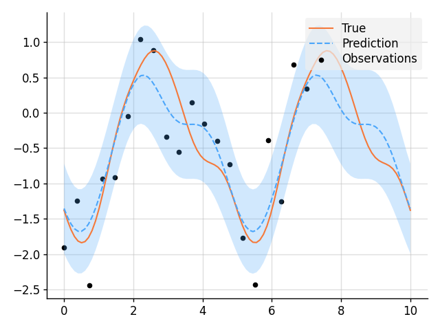
Simple Regression

import matplotlib.pyplot as plt
from wbml.plot import tweak

from stheno import B, Measure, GP, EQ, Delta

# Define points to predict at.
x = B.linspace(0, 10, 100)
x_obs = B.linspace(0, 7, 20)

# Construct a prior.
prior = Measure()
f = GP(EQ().periodic(5.0), measure=prior)  # Latent function
e = GP(Delta(), measure=prior)  # Noise
y = f + 0.5 * e

# Sample a true, underlying function and observations.
f_true, y_obs = prior.sample(f(x), y(x_obs))

# Now condition on the observations to make predictions.
post = prior | (y(x_obs), y_obs)
mean, lower, upper = post(f)(x).marginals()

# Plot result.
plt.plot(x, f_true, label="True", style="test")
plt.scatter(x_obs, y_obs, label="Observations", style="train", s=20)
plt.plot(x, mean, label="Prediction", style="pred")
plt.fill_between(x, lower, upper, style="pred")
tweak()
plt.savefig("readme_example1_simple_regression.png")
plt.show()

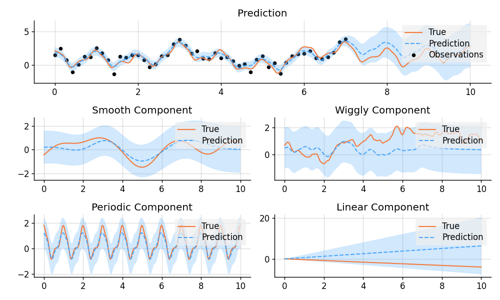
Decomposition of Prediction

import matplotlib.pyplot as plt
from wbml.plot import tweak

from stheno import Measure, GP, EQ, RQ, Linear, Delta, Exp, B

B.epsilon = 1e-10

# Define points to predict at.
x = B.linspace(0, 10, 200)
x_obs = B.linspace(0, 7, 50)

# Construct a latent function consisting of four different components.
prior = Measure()
f_smooth = GP(EQ(), measure=prior)
f_wiggly = GP(RQ(1e-1).stretch(0.5), measure=prior)
f_periodic = GP(EQ().periodic(1.0), measure=prior)
f_linear = GP(Linear(), measure=prior)

f = f_smooth + f_wiggly + f_periodic + 0.2 * f_linear

# Let the observation noise consist of a bit of exponential noise.
e_indep = GP(Delta(), measure=prior)
e_exp = GP(Exp(), measure=prior)

e = e_indep + 0.3 * e_exp

# Sum the latent function and observation noise to get a model for the observations.
y = f + 0.5 * e

# Sample a true, underlying function and observations.
(
    f_true_smooth,
    f_true_wiggly,
    f_true_periodic,
    f_true_linear,
    f_true,
    y_obs,
) = prior.sample(f_smooth(x), f_wiggly(x), f_periodic(x), f_linear(x), f(x), y(x_obs))

# Now condition on the observations and make predictions for the latent function and
# its various components.
post = prior | (y(x_obs), y_obs)

pred_smooth = post(f_smooth(x)).marginals()
pred_wiggly = post(f_wiggly(x)).marginals()
pred_periodic = post(f_periodic(x)).marginals()
pred_linear = post(f_linear(x)).marginals()
pred_f = post(f(x)).marginals()


# Plot results.
def plot_prediction(x, f, pred, x_obs=None, y_obs=None):
    plt.plot(x, f, label="True", style="test")
    if x_obs is not None:
        plt.scatter(x_obs, y_obs, label="Observations", style="train", s=20)
    mean, lower, upper = pred
    plt.plot(x, mean, label="Prediction", style="pred")
    plt.fill_between(x, lower, upper, style="pred")
    tweak()


plt.figure(figsize=(10, 6))

plt.subplot(3, 1, 1)
plt.title("Prediction")
plot_prediction(x, f_true, pred_f, x_obs, y_obs)

plt.subplot(3, 2, 3)
plt.title("Smooth Component")
plot_prediction(x, f_true_smooth, pred_smooth)

plt.subplot(3, 2, 4)
plt.title("Wiggly Component")
plot_prediction(x, f_true_wiggly, pred_wiggly)

plt.subplot(3, 2, 5)
plt.title("Periodic Component")
plot_prediction(x, f_true_periodic, pred_periodic)

plt.subplot(3, 2, 6)
plt.title("Linear Component")
plot_prediction(x, f_true_linear, pred_linear)

plt.savefig("readme_example2_decomposition.png")
plt.show()

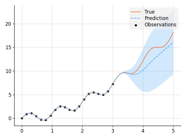
Learn a Function, Incorporating Prior Knowledge About Its Form

import matplotlib.pyplot as plt
import tensorflow as tf
import wbml.out as out
from varz.spec import parametrised, Positive
from varz.tensorflow import Vars, minimise_l_bfgs_b
from wbml.plot import tweak

from stheno.tensorflow import B, Measure, GP, EQ, Delta

# Define points to predict at.
x = B.linspace(tf.float64, 0, 5, 100)
x_obs = B.linspace(tf.float64, 0, 3, 20)


@parametrised
def model(
    vs,
    u_var: Positive = 0.5,
    u_scale: Positive = 0.5,
    e_var: Positive = 0.5,
    alpha: Positive = 1.2,
):
    prior = Measure()

    # Random fluctuation:
    u = GP(u_var * EQ() > u_scale, measure=prior)

    # Noise:
    e = GP(e_var * Delta(), measure=prior)

    # Construct model:
    f = u + (lambda x: x ** alpha)
    y = f + e

    return f, y


# Sample a true, underlying function and observations.
vs = Vars(tf.float64)
f_true = x ** 1.8 + B.sin(2 * B.pi * x)
f, y = model(vs)
post = f.measure | (f(x), f_true)
y_obs = post(f(x_obs)).sample()


def objective(vs):
    f, y = model(vs)
    evidence = y(x_obs).logpdf(y_obs)
    return -evidence


# Learn hyperparameters.
minimise_l_bfgs_b(tf.function(objective, autograph=False), vs)
f, y = model(vs)

# Print the learned parameters.
out.kv("Prior", y.display(out.format))
vs.print()

# Condition on the observations to make predictions.
post = f.measure | (y(x_obs), y_obs)
mean, lower, upper = post(f(x)).marginals()

# Plot result.
plt.plot(x, B.squeeze(f_true), label="True", style="test")
plt.scatter(x_obs, B.squeeze(y_obs), label="Observations", style="train", s=20)
plt.plot(x, mean, label="Prediction", style="pred")
plt.fill_between(x, lower, upper, style="pred")
tweak()

plt.savefig("readme_example3_parametric.png")
plt.show()

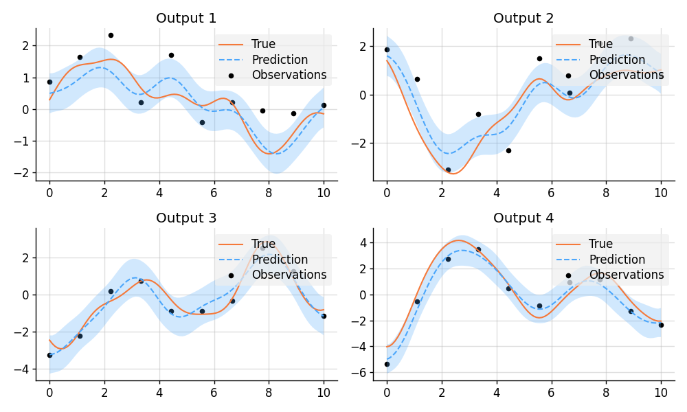
Multi-Output Regression

import matplotlib.pyplot as plt
from wbml.plot import tweak

from stheno import B, Measure, GP, EQ, Delta


class VGP:
    """A vector-valued GP."""

    def __init__(self, ps):
        self.ps = ps

    def __add__(self, other):
        return VGP([f + g for f, g in zip(self.ps, other.ps)])

    def lmatmul(self, A):
        m, n = A.shape
        ps = [0 for _ in range(m)]
        for i in range(m):
            for j in range(n):
                ps[i] += A[i, j] * self.ps[j]
        return VGP(ps)


# Define points to predict at.
x = B.linspace(0, 10, 100)
x_obs = B.linspace(0, 10, 10)

# Model parameters:
m = 2
p = 4
H = B.randn(p, m)

# Construct latent functions.
prior = Measure()
us = VGP([GP(EQ(), measure=prior) for _ in range(m)])
fs = us.lmatmul(H)

# Construct noise.
e = VGP([GP(0.5 * Delta(), measure=prior) for _ in range(p)])

# Construct observation model.
ys = e + fs

# Sample a true, underlying function and observations.
samples = prior.sample(*(p(x) for p in fs.ps), *(p(x_obs) for p in ys.ps))
fs_true, ys_obs = samples[:p], samples[p:]

# Compute the posterior and make predictions.
post = prior | (*((p(x_obs), y_obs) for p, y_obs in zip(ys.ps, ys_obs)),)
preds = [post(p(x)).marginals() for p in fs.ps]


# Plot results.
def plot_prediction(x, f, pred, x_obs=None, y_obs=None):
    plt.plot(x, f, label="True", style="test")
    if x_obs is not None:
        plt.scatter(x_obs, y_obs, label="Observations", style="train", s=20)
    mean, lower, upper = pred
    plt.plot(x, mean, label="Prediction", style="pred")
    plt.fill_between(x, lower, upper, style="pred")
    tweak()


plt.figure(figsize=(10, 6))
for i in range(4):
    plt.subplot(2, 2, i + 1)
    plt.title(f"Output {i + 1}")
    plot_prediction(x, fs_true[i], preds[i], x_obs, ys_obs[i])
plt.savefig("readme_example4_multi-output.png")
plt.show()

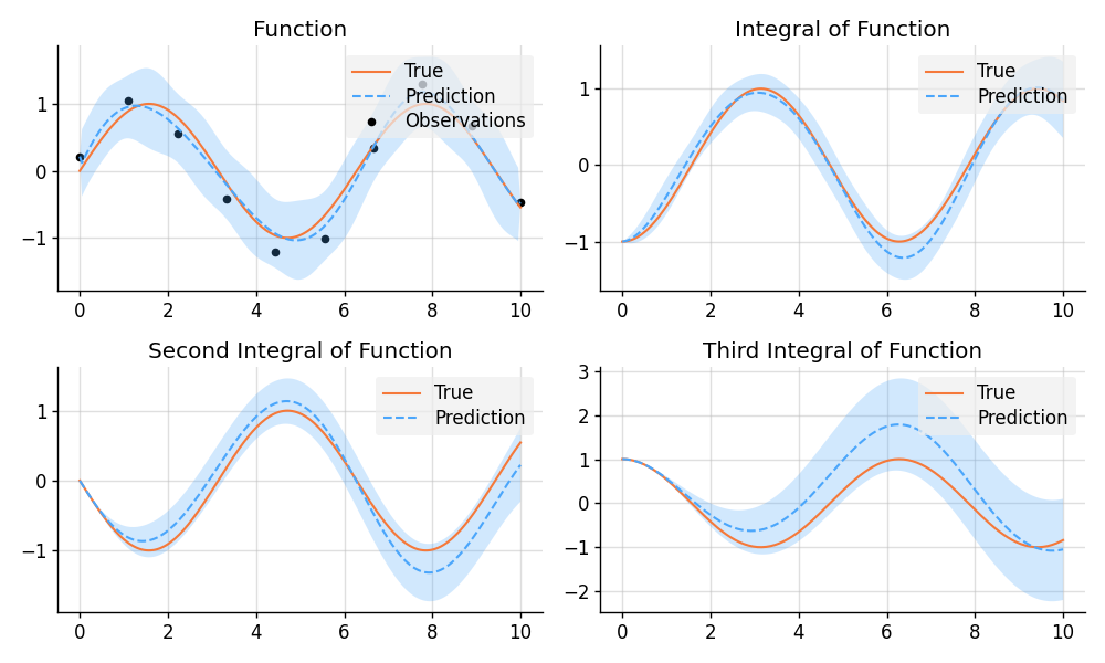
Approximate Integration

import matplotlib.pyplot as plt
import numpy as np
import tensorflow as tf
import wbml.plot

from stheno.tensorflow import B, Measure, GP, EQ, Delta

# Define points to predict at.
x = B.linspace(tf.float64, 0, 10, 200)
x_obs = B.linspace(tf.float64, 0, 10, 10)

# Construct the model.
prior = Measure()
f = 0.7 * GP(EQ(), measure=prior).stretch(1.5)
e = 0.2 * GP(Delta(), measure=prior)

# Construct derivatives.
df = f.diff()
ddf = df.diff()
dddf = ddf.diff() + e

# Fix the integration constants.
zero = B.cast(tf.float64, 0)
one = B.cast(tf.float64, 1)
prior = prior | ((f(zero), one), (df(zero), zero), (ddf(zero), -one))

# Sample observations.
y_obs = B.sin(x_obs) + 0.2 * B.randn(*x_obs.shape)

# Condition on the observations to make predictions.
post = prior | (dddf(x_obs), y_obs)

# And make predictions.
pred_iiif = post(f)(x).marginals()
pred_iif = post(df)(x).marginals()
pred_if = post(ddf)(x).marginals()
pred_f = post(dddf)(x).marginals()


# Plot result.
def plot_prediction(x, f, pred, x_obs=None, y_obs=None):
    plt.plot(x, f, label="True", style="test")
    if x_obs is not None:
        plt.scatter(x_obs, y_obs, label="Observations", style="train", s=20)
    mean, lower, upper = pred
    plt.plot(x, mean, label="Prediction", style="pred")
    plt.fill_between(x, lower, upper, style="pred")
    wbml.plot.tweak()


plt.figure(figsize=(10, 6))

plt.subplot(2, 2, 1)
plt.title("Function")
plot_prediction(x, np.sin(x), pred_f, x_obs=x_obs, y_obs=y_obs)

plt.subplot(2, 2, 2)
plt.title("Integral of Function")
plot_prediction(x, -np.cos(x), pred_if)

plt.subplot(2, 2, 3)
plt.title("Second Integral of Function")
plot_prediction(x, -np.sin(x), pred_iif)

plt.subplot(2, 2, 4)
plt.title("Third Integral of Function")
plot_prediction(x, np.cos(x), pred_iiif)

plt.savefig("readme_example5_integration.png")
plt.show()

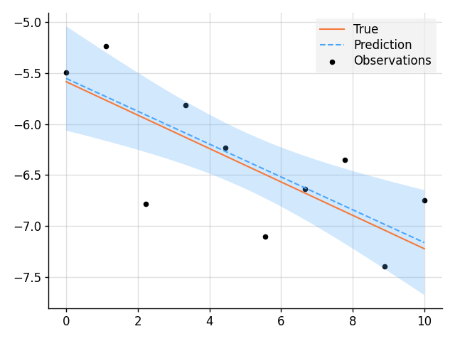
Bayesian Linear Regression

import matplotlib.pyplot as plt
import wbml.out as out
from wbml.plot import tweak

from stheno import B, Measure, GP, Delta

# Define points to predict at.
x = B.linspace(0, 10, 200)
x_obs = B.linspace(0, 10, 10)

# Construct the model.
prior = Measure()
slope = GP(1, measure=prior)
intercept = GP(5, measure=prior)
f = slope * (lambda x: x) + intercept

e = 0.2 * GP(Delta(), measure=prior)  # Noise model

y = f + e  # Observation model

# Sample a slope, intercept, underlying function, and observations.
true_slope, true_intercept, f_true, y_obs = prior.sample(
    slope(0), intercept(0), f(x), y(x_obs)
)

# Condition on the observations to make predictions.
post = prior | (y(x_obs), y_obs)
mean, lower, upper = post(f(x)).marginals()

out.kv("True slope", true_slope[0, 0])
out.kv("Predicted slope", post(slope(0)).mean[0, 0])
out.kv("True intercept", true_intercept[0, 0])
out.kv("Predicted intercept", post(intercept(0)).mean[0, 0])

# Plot result.
plt.plot(x, f_true, label="True", style="test")
plt.scatter(x_obs, y_obs, label="Observations", style="train", s=20)
plt.plot(x, mean, label="Prediction", style="pred")
plt.fill_between(x, lower, upper, style="pred")
tweak()

plt.savefig("readme_example6_blr.png")
plt.show()

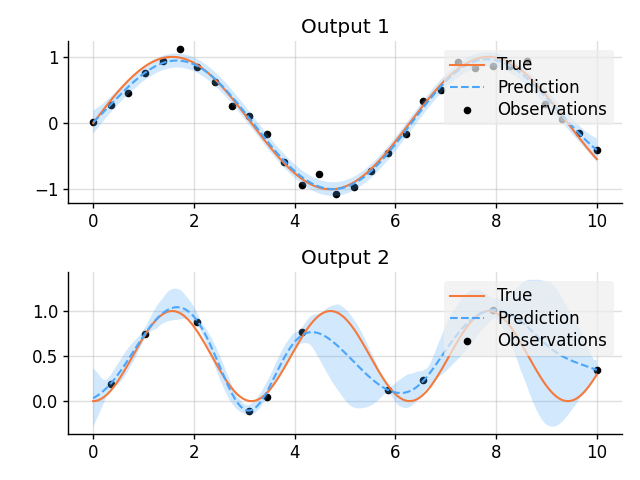
GPAR

import matplotlib.pyplot as plt
import numpy as np
import tensorflow as tf
from varz.spec import parametrised, Positive
from varz.tensorflow import Vars, minimise_l_bfgs_b
from wbml.plot import tweak

from stheno.tensorflow import B, Measure, GP, Delta, EQ

# Define points to predict at.
x = B.linspace(tf.float64, 0, 10, 200)
x_obs1 = B.linspace(tf.float64, 0, 10, 30)
inds2 = np.random.permutation(len(x_obs1))[:10]
x_obs2 = B.take(x_obs1, inds2)

# Construction functions to predict and observations.
f1_true = B.sin(x)
f2_true = B.sin(x) ** 2

y1_obs = B.sin(x_obs1) + 0.1 * B.randn(*x_obs1.shape)
y2_obs = B.sin(x_obs2) ** 2 + 0.1 * B.randn(*x_obs2.shape)


@parametrised
def model(
    vs,
    var1: Positive = 1,
    scale1: Positive = 1,
    noise1: Positive = 0.1,
    var2: Positive = 1,
    scale2: Positive = 1,
    noise2: Positive = 0.1,
):
    # Construct model for first layer:
    prior1 = Measure()
    f1 = GP(var1 * EQ() > scale1, measure=prior1)
    e1 = GP(noise1 * Delta(), measure=prior1)
    y1 = f1 + e1

    # Construct model for second layer:
    prior2 = Measure()
    f2 = GP(var2 * EQ() > scale2, measure=prior2)
    e2 = GP(noise2 * Delta(), measure=prior2)
    y2 = f2 + e2

    return f1, y1, f2, y2


def objective(vs):
    f1, y1, f2, y2 = model(vs)

    x1 = x_obs1
    x2 = B.stack(x_obs2, B.take(y1_obs, inds2), axis=1)
    evidence = y1(x1).logpdf(y1_obs) + y2(x2).logpdf(y2_obs)

    return -evidence


# Learn hyperparameters.
vs = Vars(tf.float64)
minimise_l_bfgs_b(objective, vs)

# Compute posteriors.
f1, y1, f2, y2 = model(vs)
x1 = x_obs1
x2 = B.stack(x_obs2, B.take(y1_obs, inds2), axis=1)
post1 = f1.measure | (y1(x1), y1_obs)
post2 = f2.measure | (y2(x2), y2_obs)
f1_post = post1(f1)
f2_post = post2(f2)

# Predict first output.
mean1, lower1, upper1 = f1_post(x).marginals()

# Predict second output with Monte Carlo.
samples = [
    f2_post(B.stack(x, f1_post(x).sample()[:, 0], axis=1)).sample()[:, 0]
    for _ in range(100)
]
mean2 = np.mean(samples, axis=0)
lower2 = np.percentile(samples, 2.5, axis=0)
upper2 = np.percentile(samples, 100 - 2.5, axis=0)

# Plot result.
plt.figure()

plt.subplot(2, 1, 1)
plt.title("Output 1")
plt.plot(x, f1_true, label="True", style="test")
plt.scatter(x_obs1, y1_obs, label="Observations", style="train", s=20)
plt.plot(x, mean1, label="Prediction", style="pred")
plt.fill_between(x, lower1, upper1, style="pred")
tweak()

plt.subplot(2, 1, 2)
plt.title("Output 2")
plt.plot(x, f2_true, label="True", style="test")
plt.scatter(x_obs2, y2_obs, label="Observations", style="train", s=20)
plt.plot(x, mean2, label="Prediction", style="pred")
plt.fill_between(x, lower2, upper2, style="pred")
tweak()

plt.savefig("readme_example7_gpar.png")
plt.show()

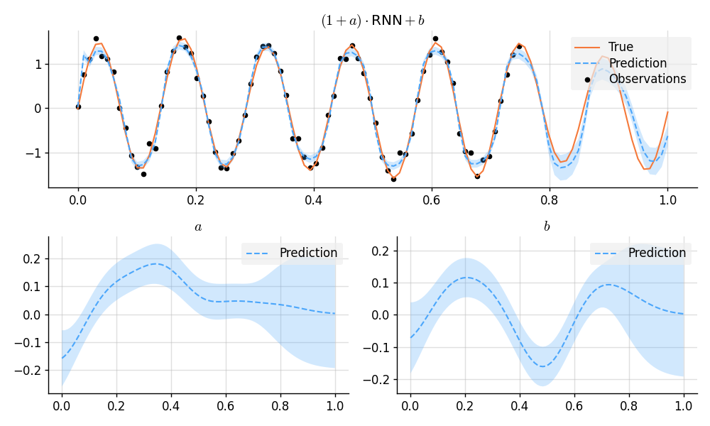
A GP-RNN Model

import matplotlib.pyplot as plt
import numpy as np
import tensorflow as tf
from varz.spec import parametrised, Positive
from varz.tensorflow import Vars, minimise_adam
from wbml.net import rnn as rnn_constructor
from wbml.plot import tweak

from stheno.tensorflow import B, Measure, GP, Delta, EQ

# Increase regularisation because we are dealing with `tf.float32`s.
B.epsilon = 1e-6

# Construct points which to predict at.
x = B.linspace(tf.float32, 0, 1, 100)[:, None]
inds_obs = B.range(0, int(0.75 * len(x)))  # Train on the first 75% only.
x_obs = B.take(x, inds_obs)

# Construct function and observations.
#   Draw random modulation functions.
a_true = GP(1e-2 * EQ().stretch(0.1))(x).sample()
b_true = GP(1e-2 * EQ().stretch(0.1))(x).sample()
#   Construct the true, underlying function.
f_true = (1 + a_true) * B.sin(2 * np.pi * 7 * x) + b_true
#   Add noise.
y_true = f_true + 0.1 * B.randn(*f_true.shape)

# Normalise and split.
f_true = (f_true - B.mean(y_true)) / B.std(y_true)
y_true = (y_true - B.mean(y_true)) / B.std(y_true)
y_obs = B.take(y_true, inds_obs)


@parametrised
def model(
    vs, a_scale: Positive = 0.1, b_scale: Positive = 0.1, noise: Positive = 0.01
):
    prior = Measure()

    # Construct an RNN.
    f_rnn = rnn_constructor(
        output_size=1, widths=(10,), nonlinearity=B.tanh, final_dense=True
    )

    # Set the weights for the RNN.
    num_weights = f_rnn.num_weights(input_size=1)
    weights = Vars(tf.float32, source=vs.get(shape=(num_weights,), name="rnn"))
    f_rnn.initialise(input_size=1, vs=weights)

    # Construct GPs that modulate the RNN.
    a = GP(1e-2 * EQ().stretch(a_scale), measure=prior)
    b = GP(1e-2 * EQ().stretch(b_scale), measure=prior)
    e = GP(noise * Delta(), measure=prior)

    # GP-RNN model:
    f_gp_rnn = (1 + a) * (lambda x: f_rnn(x)) + b
    y_gp_rnn = f_gp_rnn + e

    return f_rnn, f_gp_rnn, y_gp_rnn, a, b


def objective_rnn(vs):
    f_rnn, _, _, _, _ = model(vs)
    return B.mean((f_rnn(x_obs) - y_obs) ** 2)


def objective_gp_rnn(vs):
    _, _, y_gp_rnn, _, _ = model(vs)
    evidence = y_gp_rnn(x_obs).logpdf(y_obs)
    return -evidence


# Pretrain the RNN.
vs = Vars(tf.float32)
minimise_adam(
    tf.function(objective_rnn, autograph=False), vs, rate=1e-2, iters=1000, trace=True
)

# Jointly train the RNN and GPs.
minimise_adam(
    tf.function(objective_gp_rnn, autograph=False),
    vs,
    rate=1e-3,
    iters=1000,
    trace=True,
)

_, f_gp_rnn, y_gp_rnn, a, b = model(vs)

# Condition.
post = f_gp_rnn.measure | (y_gp_rnn(x_obs), y_obs)

# Predict and plot results.
plt.figure(figsize=(10, 6))

plt.subplot(2, 1, 1)
plt.title("$(1 + a)\\cdot {}$RNN${} + b$")
plt.plot(x, f_true, label="True", style="test")
plt.scatter(x_obs, y_obs, label="Observations", style="train", s=20)
mean, lower, upper = post(f_gp_rnn(x)).marginals()
plt.plot(x, mean, label="Prediction", style="pred")
plt.fill_between(x, lower, upper, style="pred")
tweak()

plt.subplot(2, 2, 3)
plt.title("$a$")
mean, lower, upper = post(a(x)).marginals()
plt.plot(x, mean, label="Prediction", style="pred")
plt.fill_between(x, lower, upper, style="pred")
tweak()

plt.subplot(2, 2, 4)
plt.title("$b$")
mean, lower, upper = post(b(x)).marginals()
plt.plot(x, mean, label="Prediction", style="pred")
plt.fill_between(x, lower, upper, style="pred")
tweak()

plt.savefig(f"readme_example8_gp-rnn.png")
plt.show()

Approximate Multiplication Between GPs

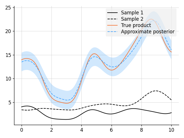
import matplotlib.pyplot as plt
from wbml.plot import tweak

from stheno import B, Measure, GP, EQ

# Define points to predict at.
x = B.linspace(0, 10, 100)

# Construct a prior.
prior = Measure()
f1 = GP(3, EQ(), measure=prior)
f2 = GP(3, EQ(), measure=prior)

# Compute the approximate product.
f_prod = f1 * f2

# Sample two functions.
s1, s2 = prior.sample(f1(x), f2(x))

# Predict.
post = prior | ((f1(x), s1), (f2(x), s2))
mean, lower, upper = post(f_prod(x)).marginals()

# Plot result.
plt.plot(x, s1, label="Sample 1", style="train")
plt.plot(x, s2, label="Sample 2", style="train", ls="--")
plt.plot(x, s1 * s2, label="True product", style="test")
plt.plot(x, mean, label="Approximate posterior", style="pred")
plt.fill_between(x, lower, upper, style="pred")
tweak()

plt.savefig("readme_example9_product.png")
plt.show()

Sparse Regression

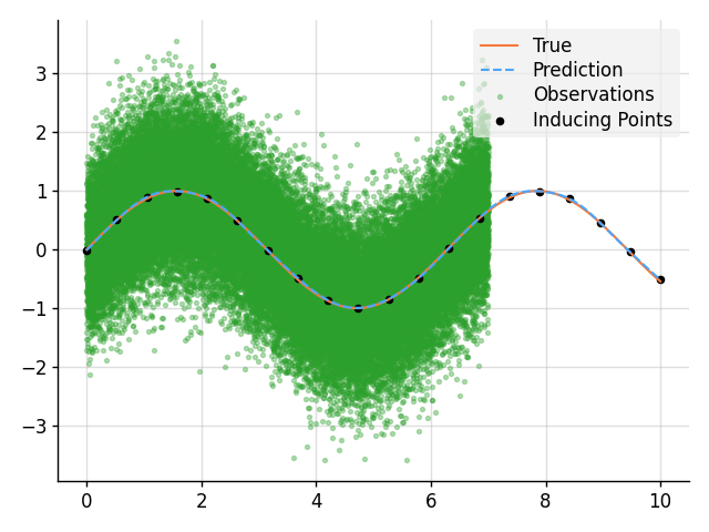
import matplotlib.pyplot as plt
import wbml.out as out
from wbml.plot import tweak

from stheno import B, Measure, GP, EQ, Delta, SparseObs

# Define points to predict at.
x = B.linspace(0, 10, 100)
x_obs = B.linspace(0, 7, 50_000)
x_ind = B.linspace(0, 10, 20)

# Construct a prior.
prior = Measure()
f = GP(EQ().periodic(2 * B.pi), measure=prior)  # Latent function.
e = GP(Delta(), measure=prior)  # Noise.
y = f + 0.5 * e

# Sample a true, underlying function and observations.
f_true = B.sin(x)
y_obs = B.sin(x_obs) + 0.5 * B.randn(*x_obs.shape)

# Now condition on the observations to make predictions.
obs = SparseObs(
    f(x_ind),  # Inducing points.
    0.5 * e,  # Noise process.
    # Observations _without_ the noise process added on.
    f(x_obs),
    y_obs,
)
out.kv("ELBO", obs.elbo(prior))
post = prior | obs
mean, lower, upper = post(f(x)).marginals()

# Plot result.
plt.plot(x, f_true, label="True", style="test")
plt.scatter(
    x_obs, y_obs, label="Observations", style="train", c="tab:green", alpha=0.35
)
plt.scatter(
    x_ind,
    obs.mu(prior)[:, 0],
    label="Inducing Points",
    style="train",
    s=20,
)
plt.plot(x, mean, label="Prediction", style="pred")
plt.fill_between(x, lower, upper, style="pred")
tweak()

plt.savefig("readme_example10_sparse.png")
plt.show()

Smoothing with Nonparametric Basis Functions

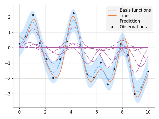
import matplotlib.pyplot as plt
from wbml.plot import tweak

from stheno import B, Measure, GP, EQ, Delta

# Define points to predict at.
x = B.linspace(0, 10, 100)
x_obs = B.linspace(0, 10, 20)

# Constuct a prior:
prior = Measure()
w = lambda x: B.exp(-(x ** 2) / 0.5)  # Window
b = [(w * GP(EQ(), measure=prior)).shift(xi) for xi in x_obs]  # Weighted basis funs
f = sum(b)  # Latent function
e = GP(Delta(), measure=prior)  # Noise
y = f + 0.2 * e  # Observation model

# Sample a true, underlying function and observations.
f_true, y_obs = prior.sample(f(x), y(x_obs))

# Condition on the observations to make predictions.
post = prior | (y(x_obs), y_obs)

# Plot result.
for i, bi in enumerate(b):
    mean, lower, upper = post(bi(x)).marginals()
    kw_args = {"label": "Basis functions"} if i == 0 else {}
    plt.plot(x, mean, style="pred2", **kw_args)
plt.plot(x, f_true, label="True", style="test")
plt.scatter(x_obs, y_obs, label="Observations", style="train", s=20)
mean, lower, upper = post(f(x)).marginals()
plt.plot(x, mean, label="Prediction", style="pred")
plt.fill_between(x, lower, upper, style="pred")
tweak()

plt.savefig("readme_example11_nonparametric_basis.png")
plt.show()