Pumas.jl

Pumas: A Pharmaceutical Modeling and Simulation toolkit

Resources

• Downloads & Install Instructions
• Documentation
• Tutorials
• Blog
• Discourse Forum

Demo: A Simple PK model

using Pumas, Plots

For reproducibility, we will set a random seed:

using Random
Random.seed!(1)

A simple one compartment oral absorption model using an analytical solution

model = @model begin
  @param   begin
    tvcl ∈ RealDomain(lower=0)
    tvv ∈ RealDomain(lower=0)
    pmoncl ∈ RealDomain(lower = -0.99)
    Ω ∈ PDiagDomain(2)
    σ_prop ∈ RealDomain(lower=0)
  end

  @random begin
    η ~ MvNormal(Ω)
  end

  @covariates wt isPM

  @pre begin
    CL = tvcl * (1 + pmoncl*isPM) * (wt/70)^0.75 * exp(η[1])
    V  = tvv * (wt/70) * exp(η[2])
  end

  @dynamics Central1
    #@dynamics begin
    #    Central' =  - (CL/V)*Central
    #end

  @derived begin
      cp = @. 1000*(Central / V)
      dv ~ @. Normal(cp, sqrt(cp^2*σ_prop))
    end
end

Develop a simple dosing regimen for a subject

ev = DosageRegimen(100, time=0, addl=4, ii=24)
s1 = Subject(id=1,  evs=ev, cvs=(isPM=1, wt=70))

Simulate a plasma concentration time profile

param = (
  tvcl = 4.0,
  tvv  = 70,
  pmoncl = -0.7,
  Ω = Diagonal([0.09,0.09]),
  σ_prop = 0.04
  )
obs = simobs(model, s1, param, obstimes=0:1:120)
plot(obs)

Generate a population of subjects

choose_covariates() = (isPM = rand([1, 0]),
              wt = rand(55:80))
pop_with_covariates = Population(map(i -> Subject(id=i, evs=ev, cvs=choose_covariates()),1:10))

Simulate into the population

obs = simobs(model, pop_with_covariates, param, obstimes=0:1:120)

and visualize the output

plot(obs)

Let's roundtrip this simulation to test our estimation routines

simdf = DataFrame(obs)
simdf.cmt .= 1
first(simdf, 6)

Read the data in to Pumas

data = read_pumas(simdf, time=:time,cvs=[:isPM, :wt])

Evaluating the results of a model fit goes through an fit --> infer --> inspect --> validate cycle

fit

julia> res = fit(model,data,param,Pumas.FOCEI())
FittedPumasModel

Successful minimization:                true

Likelihood approximation:        Pumas.FOCEI
Objective function value:            8363.13
Total number of observation records:    1210
Number of active observation records:   1210
Number of subjects:                       10

-----------------
       Estimate
-----------------
tvcl    4.7374
tvv    68.749
pmoncl -0.76408
Ω₁,₁    0.046677
Ω₂,₂    0.024126
σ_prop  0.041206
-----------------

infer

infer provides the model inference

julia> infer(res)
Calculating: variance-covariance matrix. Done.
FittedPumasModelInference

Successful minimization:                true

Likelihood approximation:        Pumas.FOCEI
Objective function value:            8363.13
Total number of observation records:    1210
Number of active observation records:   1210
Number of subjects:                       10

---------------------------------------------------
       Estimate       RSE           95.0% C.I.
---------------------------------------------------
tvcl    4.7374     10.057  [ 3.8036   ;  5.6713  ]
tvv    68.749       5.013  [61.994    ; 75.503   ]
pmoncl -0.76408    -3.9629 [-0.82342  ; -0.70473 ]
Ω₁,₁    0.046677   34.518  [ 0.015098 ;  0.078256]
Ω₂,₂    0.024126   31.967  [ 0.0090104;  0.039243]
σ_prop  0.041206    3.0853 [ 0.038714 ;  0.043698]
---------------------------------------------------

inspect

inspect gives you the model predictions, residuals and Empirical Bayes estimates

resout = DataFrame(inspect(res))

julia> first(resout, 6)
6×13 DataFrame
│ Row │ id     │ time    │ isPM  │ wt    │ pred    │ ipred   │ pred_approx │ wres     │ iwres     │ wres_approx │ ebe_1     │ ebe_2     │ ebes_approx │
│     │ String │ Float64 │ Int64 │ Int64 │ Float64 │ Float64 │ Pumas.FOCEI │ Float64  │ Float64   │ Pumas.FOCEI │ Float64   │ Float64   │ Pumas.FOCEI │
├─────┼────────┼─────────┼───────┼───────┼─────────┼─────────┼─────────────┼──────────┼───────────┼─────────────┼───────────┼───────────┼─────────────┤
│ 1   │ 1      │ 0.0     │ 1     │ 74    │ 1344.63 │ 1679.77 │ FOCEI()     │ 0.273454 │ -0.638544 │ FOCEI()     │ -0.189025 │ -0.199515 │ FOCEI()     │
│ 2   │ 1      │ 0.0     │ 1     │ 74    │ 1344.63 │ 1679.77 │ FOCEI()     │ 0.273454 │ -0.638544 │ FOCEI()     │ -0.189025 │ -0.199515 │ FOCEI()     │
│ 3   │ 1      │ 0.0     │ 1     │ 74    │ 1344.63 │ 1679.77 │ FOCEI()     │ 0.273454 │ -0.638544 │ FOCEI()     │ -0.189025 │ -0.199515 │ FOCEI()     │
│ 4   │ 1      │ 0.0     │ 1     │ 74    │ 1344.63 │ 1679.77 │ FOCEI()     │ 0.273454 │ -0.638544 │ FOCEI()     │ -0.189025 │ -0.199515 │ FOCEI()     │
│ 5   │ 1      │ 0.0     │ 1     │ 74    │ 1344.63 │ 1679.77 │ FOCEI()     │ 0.273454 │ -0.638544 │ FOCEI()     │ -0.189025 │ -0.199515 │ FOCEI()     │
│ 6   │ 1      │ 0.0     │ 1     │ 74    │ 1344.63 │ 1679.77 │ FOCEI()     │ 0.273454 │ -0.638544 │ FOCEI()     │ -0.189025 │ -0.199515 │ FOCEI()     │

Simulate from fitted model

In order to simulate from a fitted model simobs can be used. The final parameters of the fitted models are available in the coef(res)

fitparam = coef(res)

You can then pass these optimized parameters into a simobs call and pass the same dataset or simulate into a different design

ev_sd_high_dose = DosageRegimen(200, time=0, addl=4, ii=48)
s2 = Subject(id=1,  evs=ev_sd_high_dose, cvs=(isPM=1, wt=70))

obs = simobs(model, s2, fitparam, obstimes=0:1:160)
plot(obs)

Visualization

There are several plot recipes you can use to visualize your model fit. These are mainly provided by the PumasPlots.jl package (currently unregistered, add via URL).

PumasPlots provides recipes to visualize FittedPumasModels, and also has powerful grouping functionality. While some plot types are specialized for fitted models, you can use all of Plots' features by converting your result to a DataFrame (using DataFrame(inspect(res))).

• convergence(res::FittedPumasModel) - plots the optimization trajectory of all variables.

  convergence(res)
  

  

• etacov(res::FittedPumasModel) - plots the covariates of the model against the etas. Keyword arguments are described in the docstring - essentially, you can use any column in DataFrame(inspect(res)) to plot.

  etacov(res; catmap = (isPM = true,))
  

  

• resplot(res::FittedPumasModel) - plots the covariates of the model against their residuals, determined by the approximation type. Accepts many of the same kwargs as etacov.

  resplot(res; catmap = (isPM = true,))
  

  

• corrplot(empirical_bayes(res); labels) - overload of the StatsPlots corrplot, for etas.

  corrplot(empirical_bayes(res); labels = ["eta_1", "eta_2"])
  

  

Most of these plotting functions have docstrings, which can be accessed in the REPL help mode by >? resplot (for example).

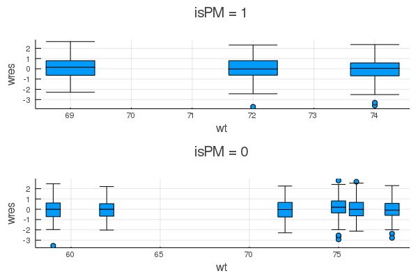
In addition to these specialized plots, PumasPlots offers powerful grouping functionality. By working with the DataFrame of your results (DataFrame(inspect(res))), you can create arbitrary plots, and by using the plot_grouped function, you can create panelled (a.k.a. grouped) plots.

df = DataFrame(inspect(res))
gdf = groupby(df, :isPM) # group by categorical covariate

plot_grouped(gdf) do subdf # `plot_grouped` will iterate through the groups of `gdf`
    boxplot(subdf.wt, subdf.wres; xlabel = :wt, ylabel = :wres, legend = :none) # you can use any arbitrary plotting function here
end