skpr

Overview

skpr is an open source design of experiments suite for generating and evaluating optimal designs in R. Here is a sampling of what skpr offers:

• Generates and evaluates D, I, A, Alias, E, T, and G optimal designs, as well as user-defined custom optimality criteria.
• Supports generation and evaluation of split/split-split/…/N-split plot designs.
• Includes parametric and Monte Carlo power evaluation functions, and supports calculating power for censored responses.
• Provides an extensible framework for the user to evaluate Monte Carlo power using their own libraries.
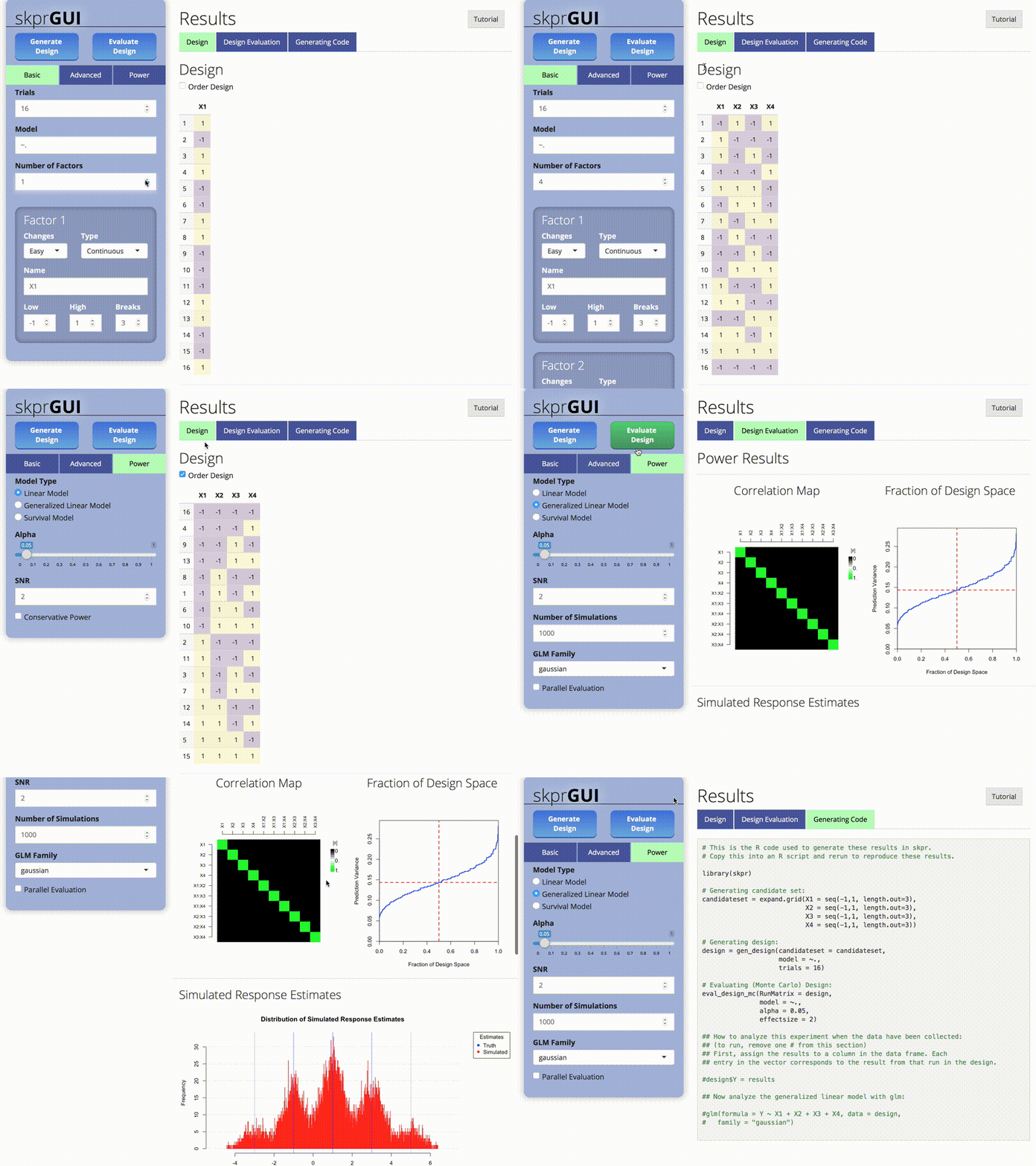
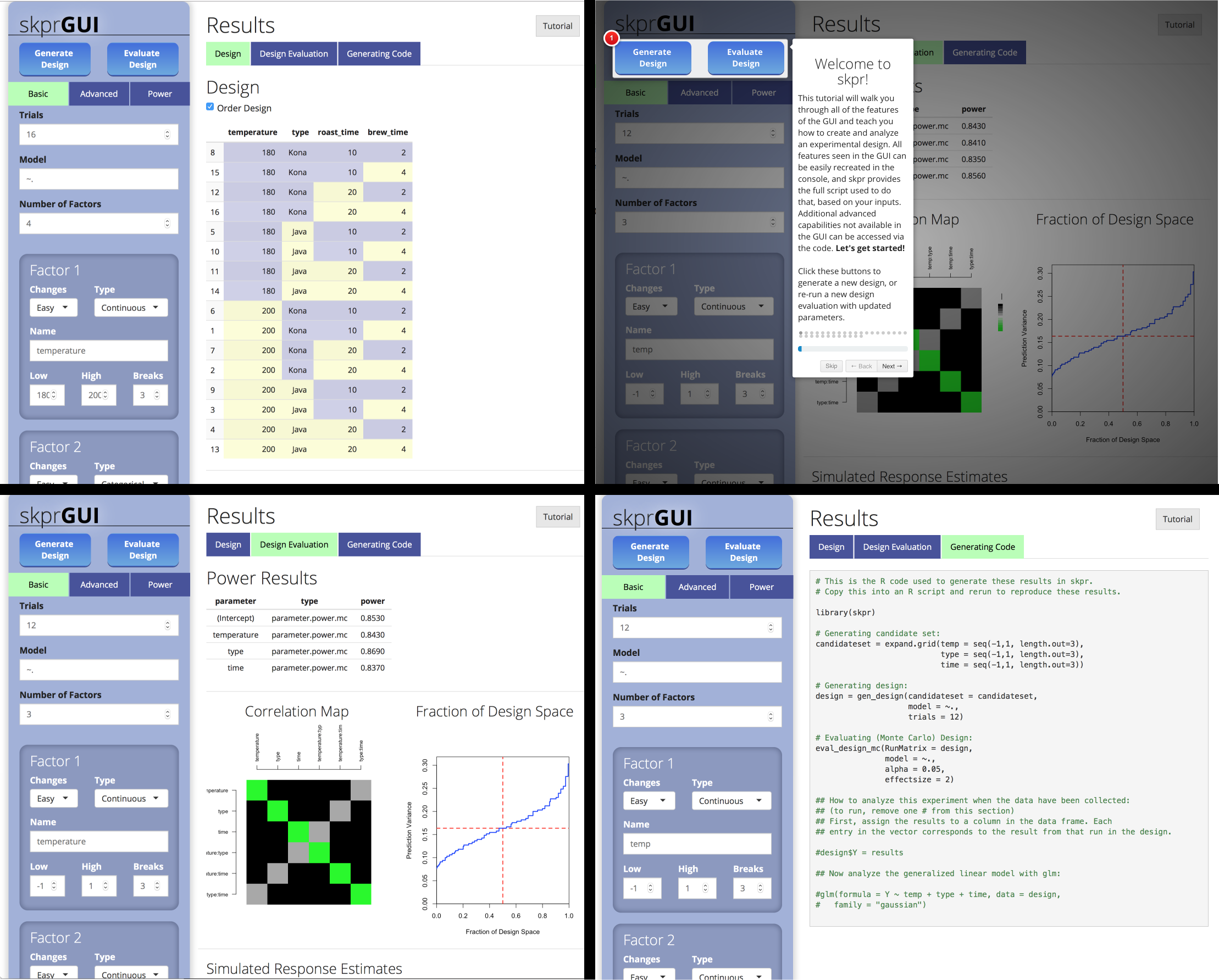
• Includes a Shiny graphical user interface, skprGUI, that auto-generates the R code used to create and evaluate the design to improve ease-of-use and enhance reproducibility.

Installation

# To install:
install.packages("skpr")

# To install the latest version from Github:
# install.packages("devtools")
devtools::install_github("tylermorganwall/skpr")

Functions

• gen_design() generates optimal designs from a candidate set, given a model and the desired number of runs.
• eval_design() evaluates power parametrically for linear models, for normal and split-plot designs.
• eval_design_mc() evaluates power with a Monte Carlo simulation, for linear and generalized linear models. This function also supports calculating power for split-plot designs using REML.
• eval_design_survival_mc() evaluates power with a Monte Carlo simulation, allowing the user to specify a point at which the data is censored.
• eval_design_custom_mc() allows the user to import their own libraries and use the Monte Carlo framework provided by skpr to calculate power.
• skprGUI() and skprGUIbrowser() opens up the GUI in either R Studio or an external browser.

If addition, the package offers two functions to generate common plots related to designs:

• plot_correlations() generates a color map of correlations between variables.
• plot_fds() generates the fraction of design space plot for a given design.

##skprGUI

skprGUI provides an graphical user interface to access all of the main features of skpr. An interactive tutorial is provided to familiarize the user with the available functionality. Type skprGUI() or skprGUIbrowser() to begin. Screenshots:

Usage

library(skpr)

#Generate a candidate set of all potential design points to be considered in the experiment
#The hypothetical experiment is determining what affects the caffeine content in coffee
candidate_set = expand.grid(temp = c(80,90,100), 
                            type = c("Kona","Java"),
                            beansize = c("Large","Medium","Small"))
candidate_set
#>    temp type beansize
#> 1    80 Kona    Large
#> 2    90 Kona    Large
#> 3   100 Kona    Large
#> 4    80 Java    Large
#> 5    90 Java    Large
#> 6   100 Java    Large
#> 7    80 Kona   Medium
#> 8    90 Kona   Medium
#> 9   100 Kona   Medium
#> 10   80 Java   Medium
#> 11   90 Java   Medium
#> 12  100 Java   Medium
#> 13   80 Kona    Small
#> 14   90 Kona    Small
#> 15  100 Kona    Small
#> 16   80 Java    Small
#> 17   90 Java    Small
#> 18  100 Java    Small

#Generate the design (default D-optimal)
design = gen_design(candidateset = candidate_set, 
                    model = ~temp + type + beansize,
                    trials=12)
design
#>    temp type beansize
#> 1    80 Java   Medium
#> 2   100 Java    Large
#> 3   100 Java    Small
#> 4    80 Java    Large
#> 5    80 Kona   Medium
#> 6    80 Kona    Small
#> 7   100 Kona    Small
#> 8   100 Kona   Medium
#> 9    80 Kona    Large
#> 10  100 Java   Medium
#> 11  100 Kona    Large
#> 12   80 Java    Small

#Evaluate power for the design with an allowable type-I error of 5% (default)
eval_design(design)
#>     parameter            type     power
#> 1 (Intercept)    effect.power 0.8424665
#> 2        temp    effect.power 0.8424665
#> 3        type    effect.power 0.8424665
#> 4    beansize    effect.power 0.5165386
#> 5 (Intercept) parameter.power 0.8424665
#> 6        temp parameter.power 0.8424665
#> 7       type1 parameter.power 0.8424665
#> 8   beansize1 parameter.power 0.5593966
#> 9   beansize2 parameter.power 0.5593966
#> ============Evaluation Info============
#> • Alpha = 0.05 • Trials = 12 • Blocked = FALSE
#> • Evaluating Model = ~temp + type + beansize
#> • Anticipated Coefficients = c(1.000, 1.000, 1.000, 1.000, -1.000)

#Evaluate power for the design using a Monte Carlo simulation. 
#Here, we set the effect size (here, the signal-to-noise ratio) to 1.5.
eval_design_mc(design, effectsize=1.5)
#>     parameter               type power
#> 1 (Intercept)    effect.power.mc 0.600
#> 2        temp    effect.power.mc 0.612
#> 3        type    effect.power.mc 0.610
#> 4    beansize    effect.power.mc 0.316
#> 5 (Intercept) parameter.power.mc 0.600
#> 6        temp parameter.power.mc 0.612
#> 7       type1 parameter.power.mc 0.610
#> 8   beansize1 parameter.power.mc 0.359
#> 9   beansize2 parameter.power.mc 0.354
#> ===========Evaluation Info============
#> • Alpha = 0.05 • Trials = 12 • Blocked = FALSE
#> • Evaluating Model = ~temp + type + beansize
#> • Anticipated Coefficients = c(0.750, 0.750, 0.750, 0.750, -0.750)

#Evaluate power for the design using a Monte Carlo simulation, for a non-normal response. 
#Here, we also increase the number of simululations to improve the precision of the results.
eval_design_mc(design, nsim=5000, glmfamily = "poisson", effectsize=c(2,6))
#>     parameter               type  power
#> 1 (Intercept)    effect.power.mc 0.9968
#> 2        temp    effect.power.mc 0.9826
#> 3        type    effect.power.mc 0.9832
#> 4    beansize    effect.power.mc 0.8502
#> 5 (Intercept) parameter.power.mc 0.9968
#> 6        temp parameter.power.mc 0.9826
#> 7       type1 parameter.power.mc 0.9832
#> 8   beansize1 parameter.power.mc 0.8842
#> 9   beansize2 parameter.power.mc 0.7052
#> ============Evaluation Info============
#> • Alpha = 0.05 • Trials = 12 • Blocked = FALSE
#> • Evaluating Model = ~temp + type + beansize
#> • Anticipated Coefficients = c(1.242, 0.549, 0.549, 0.549, -0.549)

#skpr was designed to operate with the pipe (%>%) in mind. 
#Here is an example of an entire design of experiments analysis in three lines:

expand.grid(temp = c(80,90,100), type = c("Kona","Java"), beansize = c("Large","Medium","Small")) %>%
  gen_design(model = ~temp + type + beansize + beansize:type + I(temp^2), trials=24, optimality="I") %>%
  eval_design_mc()
#>          parameter               type power
#> 1      (Intercept)    effect.power.mc 0.912
#> 2             temp    effect.power.mc 0.927
#> 3             type    effect.power.mc 0.997
#> 4         beansize    effect.power.mc 0.935
#> 5        I(temp^2)    effect.power.mc 0.637
#> 6    type:beansize    effect.power.mc 0.913
#> 7      (Intercept) parameter.power.mc 0.912
#> 8             temp parameter.power.mc 0.927
#> 9            type1 parameter.power.mc 0.997
#> 10       beansize1 parameter.power.mc 0.917
#> 11       beansize2 parameter.power.mc 0.913
#> 12       I(temp^2) parameter.power.mc 0.637
#> 13 type1:beansize1 parameter.power.mc 0.899
#> 14 type1:beansize2 parameter.power.mc 0.902
#> ==============Evaluation Info==============
#> • Alpha = 0.05 • Trials = 24 • Blocked = FALSE
#> • Evaluating Model = ~temp + type + beansize + type:beansize + I(temp^2)
#> • Anticipated Coefficients = c(1.000, 1.000, 1.000, 1.000, -1.000, 1.000, 1.000, -1.000)