summarytools

The following vignettes complement this page:

Recommendations for Using summarytools With Rmarkdown
Introduction to summarytools – Contents similar to this page (minus installation instructions), with fancier table stylings.

1. Overview

summarytools is a an R package for data exploration and simple reporting.

Four functions are at its core:

Function	Description
freq()	Frequency Tables featuring counts, proportions, as well as missing data information
ctable()	Cross-Tabulations (joint frequencies) between pairs of discrete variables featuring marginal sums as well as row, column or total proportions
descr()	Descriptive (Univariate) Statistics for numerical data featuring common measures of central tendency and dispersion
dfSummary()	Extensive Data Frame Summaries featuring type-specific information for all variables in a data frame: univariate statistics and/or frequency distributions, bar charts or histograms, as well as missing data counts. Very useful to quickly detect anomalies and identify trends at a glance

1.1 Motivation

The package was developed with the following objectives in mind:

• Provide a coherent set of easy-to-use descriptive functions that are akin to those included in commercial statistical software suites such as SAS, SPSS, and Stata
• Offer flexibility in terms of output format & content
• Integrate well with commonly used software & tools for reporting (the RStudio IDE, Rmarkdown, and knitr) while also allowing for standalone, simple report generation from any R interface

On a more personal level, I simply wish to share with the R community and the scientific community at large the functions I first developed for myself, that I ultimately realized would benefit a lot of people who are looking for the same thing I was seeking in the first place.

Support summarytools’ Development With a Small Donation

Some package developers and maintainers get paid to do exactly that. They may also work in teams. This is not my case. Seeing the package grow in popularity was and still is in itself a rewarding experience, but I won’t lie; keeping up with the maintenance, feature requests and other features I have in mind takes more time than I can afford.

So if you find summarytools useful and want to support its development, please consider making a small donation using the PayPal button. In exchange, on top of contributing to the package and helping out other data scientists, students and researchers, you’ll get:

• My sincere gratitude
• Your name listed in the Sponsors section of this page
• My personal commitment to dedicate more time to the package’s development

1.2 Redirecting Outputs

Results can be

• Displayed in the R console as plain text
• Rendered as html and shown in a Web browser or in RStudio’s Viewer pane
• Written to, or appended to plain text, markdown, or html files

1.3 Other Characteristics

• Pipe-Friendly:
  • The %>% and %$% operators from the magrittr package are supported
  • The %>>% operator from the pipeR package is also supported
• Multilingual:
  • Built-in translations exist for French, Portuguese, Spanish, Russian and Turkish
  • Users can easily add custom translations or modify existing sets of translations as needed
• Weights-enabled: except for dfSummary(), all core functions support sampling weights
• Flexible:
  • Default values for most function arguments can be modified using st_options(); this simplifies coding and minimizes redundancy
  • Pander options can be used for text / markdown tables
  • Base R’s format() parameters are supported; this is especially useful to set thousands separators, among several other possibilities
  • Bootstrap CSS used by default with html outputs, and user-defined classes can be added at will

1.4 Installing summarytools

Required Software

Additional software is used by summarytools to fine-tune graphics as well as offer interactive features. If installing summarytools for the first time, click on the link corresponding to your Operating System to get detailed instructions. Note that on Windows, no additional software is required.

Mac OS X
Ubuntu / Debian / Mint
Older Ubuntu (14 and 16)
Fedora / Red Hat / CentOS
Solaris

Installing From GitHub

This is the recommended method, as some minor fixes and improvements are regularly added.

install.packages("remotes") # Using devtools is also possible
library(remotes)
install_github("rapporter/pander") # Necessary for optimal results!
install_github("dcomtois/summarytools")

Installing From CRAN

CRAN versions are stable but are not updated as often as the GitHub versions.

install.packages("summarytools")

1.5 Latest Features (versions 0.9.7 and 0.9.8)

• Performance and formatting improvements
• The stview() function which ensures the package’s own view() method
  is used (avoiding potential conflicts with other packages’ versions of that method)
• Several other features (see NEWS.md or try news(package="summarytools"))

2. The Four Core Functions

2.1 Frequency Tables With freq()

The freq() function generates frequency tables with counts, proportions, as well as missing data information.

freq(iris$Species, plain.ascii = FALSE, style = "rmarkdown")

Frequencies

iris$Species
Type: Factor

	Freq	% Valid	% Valid Cum.	% Total	% Total Cum.
setosa	50	33.33	33.33	33.33	33.33
versicolor	50	33.33	66.67	33.33	66.67
virginica	50	33.33	100.00	33.33	100.00
<NA>	0			0.00	100.00
Total	150	100.00	100.00	100.00	100.00

In this first example, the plain.ascii and style arguments were specified. However, since we have defined them globally for this document using st_options(), they are redundant and will be omitted from hereon.

2.1.1 Formatting Numbers With format()’s Arguments

As of version 0.9.8, it is possible to use base R’s format() parameters when calling freq() or any other core function. Some of the most useful are big.mark, which inserts thousands separators, and decimal.mark, which allows using commas instead of dots as decimal separator (useful in several locales). Note that decimal marks can also be set globally with the R option OutDec (e.g. options(OutDec = ",")). The formatting is applied in the heading section as well as in the results tables:

set.seed(2835)
Random_numbers <- sample(c(5e3, 5e4, 5e5), size = 1e4, replace = TRUE, prob = c(.12, .36, .52))
freq(Random_numbers, big.mark = ",", cumul = FALSE, headings = FALSE)

## setting plain.ascii to FALSE

	Freq	% Valid	% Total
5,000	1,237	12.37	12.37
50,000	3,605	36.05	36.05
500,000	5,158	51.58	51.58
<NA>	0		0.00
Total	10,000	100.00	100.00

# We can also use format() arguments with print / view
print(freq(Random_numbers, cumul = FALSE, headings = FALSE), big.mark = " ", decimal.mark = ".")

## setting plain.ascii to FALSE

	Freq	% Valid	% Total
5 000	1 237	12.37	12.37
50 000	3 605	36.05	36.05
500 000	5 158	51.58	51.58
<NA>	0		0.00
Total	10 000	100.00	100.00

2.1.2 Ignoring Missing Data

The report.nas argument can be set to FALSE in order to ignore missing values (NA’s). Doing so has the following effects on the resulting table:

1. The <NA> row is omitted
2. The % Total and % Total Cum. (cumulative) columns are also omitted
3. The % Valid column simply becomes %
4. The % Valid Cum. column simply becomes % Cum.

freq(iris$Species, report.nas = FALSE, headings = FALSE)

## setting plain.ascii to FALSE

	Freq	%	% Cum.
setosa	50	33.33	33.33
versicolor	50	33.33	66.67
virginica	50	33.33	100.00
Total	150	100.00	100.00

Note that the headings = FALSE parameter suppresses the heading section. (The heading section consists of a title, as well as various metadata elements: object names, labels, by-groups, and so on.

2.1.3 Minimal Frequency Tables

By “switching off” all optional elements, a much simpler table will be produced:

freq(iris$Species, report.nas = FALSE, totals = FALSE, 
     cumul = FALSE, headings = FALSE)

## setting plain.ascii to FALSE

	Freq	%
setosa	50	33.33
versicolor	50	33.33
virginica	50	33.33

2.1.4 Multiple Frequency Tables

To generate frequency tables for all variables in a data frame, one could use lapply(). However, this is not required since freq() handles whole data frames, too:

freq(tobacco)

To avoid cluttering the results, numerical columns having more than 25 distinct values are ignored. This threshold of 25 can be changed by using st_options(); for example, to change it to 10, we’d use st_options(freq.ignore.threshold = 10).

Note: the tobacco data frame contains simulated data and is included in the package. Another simulated data frame is included: exams. Both have French versions (tabagisme, examens).

2.1.5 Subsetting (Filtering) Frequency Tables

The rows parameter allows subsetting frequency tables; we can use this parameter in different ways:

• To filter rows by their order of appearance, we use a numerical vector; rows = 1:10 will show the frequencies for the first 10 values only
• To filter rows by name, we can use
  • a character vector specifying the exact row names we wish to keep in the results
  • a single character string which will be used as a regular expression to select the matching column(s); see ?regex for more information on regular expressions

Used in combination with the order argument, the subsetting feature can be quite practical. For a character variable containing a large number of distinct values, showing only the most frequent is easily done:

freq(tobacco$disease, order = "freq", rows = 1:5, headings = FALSE)

## setting plain.ascii to FALSE

	Freq	% Valid	% Valid Cum.	% Total	% Total Cum.
Hypertension	36	16.22	16.22	3.60	3.60
Cancer	34	15.32	31.53	3.40	7.00
Cholesterol	21	9.46	40.99	2.10	9.10
Heart	20	9.01	50.00	2.00	11.10
Pulmonary	20	9.01	59.01	2.00	13.10
(Other)	91	40.99	100.00	9.10	22.20
<NA>	778			77.80	100.00
Total	1000	100.00	100.00	100.00	100.00

Instead of "freq", we can use "-freq" to reverse the ordering and get results ranked from lowest to highest in frequency.

To account for the frequencies of unshown values, the “(Other)” row is automatically added.

2.1.6 Collapsible Sections

When generating html results, use the collapse = TRUE argument with print() or view() to get collapsible sections; clicking on the variable name in the heading section will collapse / reveal the frequency table (results not shown).

view(freq(tobacco), collapse = TRUE)

2.2 Cross-Tabulations with ctable()

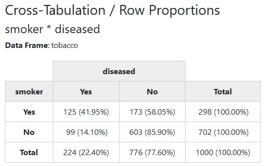
ctable() generates cross-tabulations (joint frequencies) for pairs of categorical variables.

Since markdown does not support multiline table headings (but does accept html code), we’ll use the html rendering feature for this section.

Using the tobacco data frame, we’ll cross-tabulate the two categorical variables smoker and diseased.

print(ctable(x = tobacco$smoker, y = tobacco$diseased, prop = "r"),
      method = "render")

2.2.1 Row, Column or Total Proportions

Row proportions are shown by default. To display column or total proportions, use prop = "c" or prop = "t", respectively. To omit proportions altogether, use prop = "n".

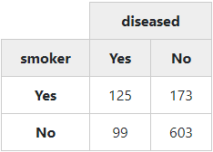
2.2.2 Minimal Cross-Tabulations

By “switching off” all optional features, we get a simple “2 x 2” table:

with(tobacco, 
     print(ctable(x = smoker, y = diseased, prop = 'n',
                  totals = FALSE, headings = FALSE),
           method = "render"))

2.2.3 Chi-Square (𝛘²), Odds Ratio and Risk Ratio

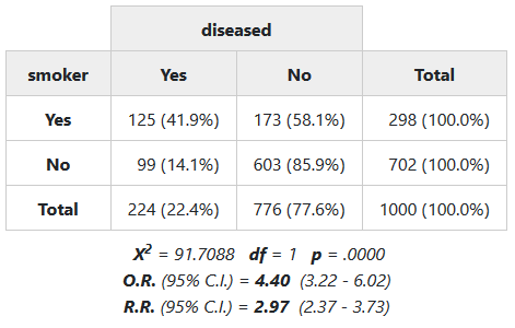
To display the chi-square statistic, set chisq = TRUE. For 2 x 2 tables, use OR and RR to show odds ratio and risk ratio (also called relative risk), respectively. Those can be set to TRUE, in which case 95% confidence intervals will be shown; to use alternate confidence levels, use for example OR = .90.

To show how pipes can be used with summarytools, we’ll use magrittr’s %$% and %>% operators:

library(magrittr)
tobacco %$%  # Acts like with(tobacco, ...)
  ctable(smoker, diseased,
         chisq = TRUE, OR = TRUE, RR = TRUE,
         headings = FALSE) %>%
  print(method = "render")

2.3 Descriptive Statistics With descr()

descr() generates descriptive / univariate statistics, i.e. common central tendency statistics and measures of dispersion. It accepts single vectors as well as data frames; in the latter case, all non-numerical columns are ignored, with a message to that effect.

descr(iris)

Descriptive Statistics

iris
N: 150

	Petal.Length	Petal.Width	Sepal.Length	Sepal.Width
Mean	3.76	1.20	5.84	3.06
Std.Dev	1.77	0.76	0.83	0.44
Min	1.00	0.10	4.30	2.00
Q1	1.60	0.30	5.10	2.80
Median	4.35	1.30	5.80	3.00
Q3	5.10	1.80	6.40	3.30
Max	6.90	2.50	7.90	4.40
MAD	1.85	1.04	1.04	0.44
IQR	3.50	1.50	1.30	0.50
CV	0.47	0.64	0.14	0.14
Skewness	-0.27	-0.10	0.31	0.31
SE.Skewness	0.20	0.20	0.20	0.20
Kurtosis	-1.42	-1.36	-0.61	0.14
N.Valid	150.00	150.00	150.00	150.00
Pct.Valid	100.00	100.00	100.00	100.00

2.3.1 Transposing and Selecting Statistics

Results can be transposed by using transpose = TRUE, and statistics can be selected using the stats argument:

descr(iris, stats = c("mean", "sd"), transpose = TRUE, headings = FALSE)

	Mean	Std.Dev
Petal.Length	3.76	1.77
Petal.Width	1.20	0.76
Sepal.Length	5.84	0.83
Sepal.Width	3.06	0.44

See ?descr for a list of all available statistics. Special values “all”, “fivenum”, and “common” are also valid values for the stats argument. The default value is “all”.

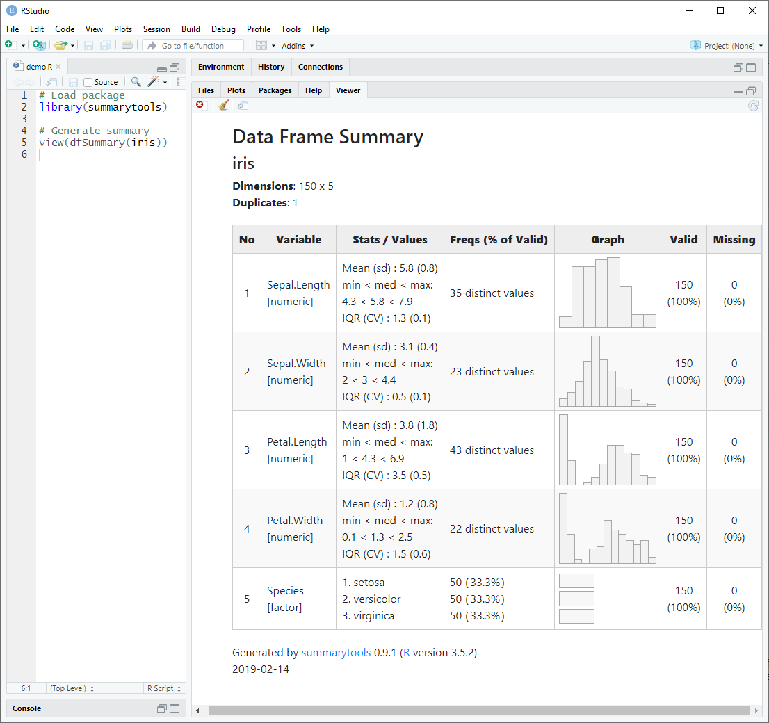
2.4 Data Frame Summaries With dfSummary()

dfSummary() creates a summary table with statistics, frequencies and graphs for all variables in a data frame. The information displayed is type-specific (character, factor, numeric, date) and also varies according to the number of distinct values.

To see the results in RStudio’s Viewer (or in the default Web browser if working in another IDE or from a terminal window), we use the view() function:

view(dfSummary(iris))

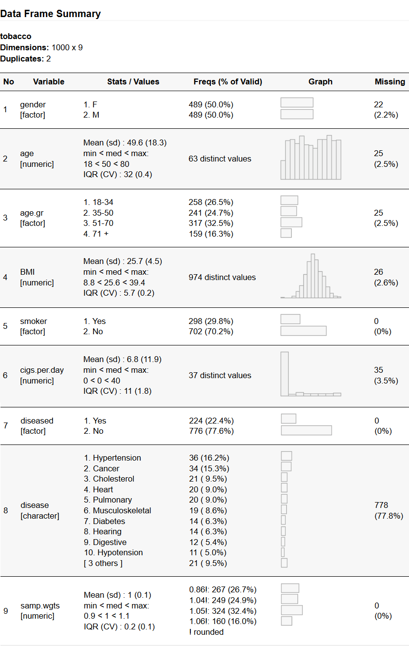
2.4.1 Using dfSummary() in Rmarkdown Documents

When using dfSummary() in Rmarkdown documents, it is generally a good idea to exclude a column or two to avoid margin overflow. Since the Valid and Missing columns are redundant, we can drop either one of them.

dfSummary(tobacco, plain.ascii = FALSE, style = "grid", 
          graph.magnif = 0.75, valid.col = FALSE, tmp.img.dir = "/tmp")

The tmp.img.dir parameter is mandatory when generating dfSummaries in Rmarkdown documents, except for html rendering. The explanation for this can be found further below.

2.4.2 Advanced Features

The dfSummary() function also

• Reports the number of duplicate records in the heading section
• Detects UPC/EAN codes (barcode numbers) and doesn’t calculate irrelevant statistics for them
• Detects email addresses and reports counts of valid, invalid and duplicate addresses

2.4.3 Excluding Columns

Although most columns can be excluded using the function’s parameters, it is also possible to delete them with the following syntax (results not shown):

dfs <- dfSummary(iris)
dfs$Variable <- NULL # This deletes the "Variable" column

3. Grouped Statistics Using stby()

To produce optimal results, summarytools has its own version of the base by() function. It’s called stby(), and we use it exactly as we would by():

(iris_stats_by_species <- stby(data = iris, 
                               INDICES = iris$Species, 
                               FUN = descr, stats = "common", transpose = TRUE))

## Non-numerical variable(s) ignored: Species

Descriptive Statistics

iris
Group: Species = setosa
N: 50

	Mean	Std.Dev	Min	Median	Max	N.Valid	Pct.Valid
Petal.Length	1.46	0.17	1.00	1.50	1.90	50.00	100.00
Petal.Width	0.25	0.11	0.10	0.20	0.60	50.00	100.00
Sepal.Length	5.01	0.35	4.30	5.00	5.80	50.00	100.00
Sepal.Width	3.43	0.38	2.30	3.40	4.40	50.00	100.00

Group: Species = versicolor
N: 50

	Mean	Std.Dev	Min	Median	Max	N.Valid	Pct.Valid
Petal.Length	4.26	0.47	3.00	4.35	5.10	50.00	100.00
Petal.Width	1.33	0.20	1.00	1.30	1.80	50.00	100.00
Sepal.Length	5.94	0.52	4.90	5.90	7.00	50.00	100.00
Sepal.Width	2.77	0.31	2.00	2.80	3.40	50.00	100.00

Group: Species = virginica
N: 50

	Mean	Std.Dev	Min	Median	Max	N.Valid	Pct.Valid
Petal.Length	5.55	0.55	4.50	5.55	6.90	50.00	100.00
Petal.Width	2.03	0.27	1.40	2.00	2.50	50.00	100.00
Sepal.Length	6.59	0.64	4.90	6.50	7.90	50.00	100.00
Sepal.Width	2.97	0.32	2.20	3.00	3.80	50.00	100.00

3.1 Special Case of descr() with stby()

When used to produce split-group statistics for a single variable, stby() assembles everything into a single table instead of displaying a series of one-column tables.

with(tobacco, stby(data = BMI, INDICES = age.gr, 
                   FUN = descr, stats = c("mean", "sd", "min", "med", "max")))

Descriptive Statistics

BMI by age.gr
Data Frame: tobacco
N: 258

	18-34	35-50	51-70	71 +
Mean	23.84	25.11	26.91	27.45
Std.Dev	4.23	4.34	4.26	4.37
Min	8.83	10.35	9.01	16.36
Median	24.04	25.11	26.77	27.52
Max	34.84	39.44	39.21	38.37

3.2 Using stby() With ctable()

The syntax is a little trickier for this combination, so here is an example (results not shown):

stby(list(x = tobacco$smoker, y = tobacco$diseased), 
     INDICES = tobacco$gender, FUN = ctable)

# or equivalently
with(tobacco, 
     stby(list(x = smoker, y = diseased), 
          INDICES = gender, FUN = ctable))

4. Grouped Statistics Using dplyr::group_by()

To create grouped statistics with freq(), descr() or dfSummary(), it is possible to use dplyr’s group_by() as an alternative to stby(). Syntactic differences aside, one key distinction is that group_by() considers NA values on the grouping variable(s) as a valid category, albeit with a warning message suggesting the use of forcats::fct_explicit_na to make NA’s explicit in factors. Following this advice, we get:

library(dplyr)
tobacco$gender %<>% forcats::fct_explicit_na()
tobacco %>% group_by(gender) %>% descr(stats = "fivenum")

## Non-numerical variable(s) ignored: age.gr, smoker, diseased, disease

Descriptive Statistics

tobacco
Group: gender = F
N: 489

	age	BMI	cigs.per.day	samp.wgts
Min	18.00	9.01	0.00	0.86
Q1	34.00	22.98	0.00	0.86
Median	50.00	25.87	0.00	1.04
Q3	66.00	29.48	10.50	1.05
Max	80.00	39.44	40.00	1.06

Group: gender = M
N: 489

	age	BMI	cigs.per.day	samp.wgts
Min	18.00	8.83	0.00	0.86
Q1	34.00	22.52	0.00	0.86
Median	49.50	25.14	0.00	1.04
Q3	66.00	27.96	11.00	1.05
Max	80.00	36.76	40.00	1.06

Group: gender = (Missing)
N: 22

	age	BMI	cigs.per.day	samp.wgts
Min	19.00	20.24	0.00	0.86
Q1	36.00	24.97	0.00	1.04
Median	55.50	27.16	0.00	1.05
Q3	64.00	30.23	10.00	1.05
Max	80.00	32.43	28.00	1.06

5. Creating Tidy Tables With tb()

When generating freq() or descr() tables, it is possible to turn the results into “tidy” tables with the use of the tb() function (think of tb as a diminutive for tibble). For example:

library(magrittr)
iris %>% descr(stats = "common") %>% tb()

## # A tibble: 4 x 8
##   variable      mean    sd   min   med   max n.valid pct.valid
##   <chr>        <dbl> <dbl> <dbl> <dbl> <dbl>   <dbl>     <dbl>
## 1 Petal.Length  3.76 1.77    1    4.35   6.9     150       100
## 2 Petal.Width   1.20 0.762   0.1  1.3    2.5     150       100
## 3 Sepal.Length  5.84 0.828   4.3  5.8    7.9     150       100
## 4 Sepal.Width   3.06 0.436   2    3      4.4     150       100

iris$Species %>% freq(cumul = FALSE, report.nas = FALSE) %>% tb()

## setting plain.ascii to FALSE

## # A tibble: 3 x 3
##   Species     freq   pct
##   <fct>      <dbl> <dbl>
## 1 setosa        50  33.3
## 2 versicolor    50  33.3
## 3 virginica     50  33.3

By definition, no total rows are part of tidy tables, and the row names are converted to a regular column. Note that for displaying tibbles using Rmarkdown, the knitr chunk option ‘results’ should be set to “markup” instead of “asis”.

5.1 Tidy Split-Group Statistics

Here are some examples showing how lists created using stby() or group_by() can be transformed into tidy tibbles.

grouped_descr <- stby(data = exams, INDICES = exams$gender, 
                      FUN = descr, stats = "common")
grouped_descr %>% tb()

## # A tibble: 12 x 9
##    gender variable   mean    sd   min   med   max n.valid pct.valid
##    <fct>  <chr>     <dbl> <dbl> <dbl> <dbl> <dbl>   <dbl>     <dbl>
##  1 Girl   economics  72.5  7.79  62.3  70.2  89.6      14      93.3
##  2 Girl   english    73.9  9.41  58.3  71.8  93.1      14      93.3
##  3 Girl   french     71.1 12.4   44.8  68.4  93.7      14      93.3
##  4 Girl   geography  67.3  8.26  50.4  67.3  78.9      15     100  
##  5 Girl   history    71.2  9.17  53.9  72.9  86.4      15     100  
##  6 Girl   math       73.8  9.03  55.6  74.8  86.3      14      93.3
##  7 Boy    economics  75.2  9.40  60.5  71.7  94.2      15     100  
##  8 Boy    english    77.8  5.94  69.6  77.6  90.2      15     100  
##  9 Boy    french     76.6  8.63  63.2  74.8  94.7      15     100  
## 10 Boy    geography  73   12.4   47.2  71.2  96.3      14      93.3
## 11 Boy    history    74.4 11.2   54.4  72.6  93.5      15     100  
## 12 Boy    math       73.3  9.68  60.5  72.2  93.2      14      93.3

The order parameter controls row ordering:

grouped_descr %>% tb(order = 2)

## # A tibble: 12 x 9
##    gender variable   mean    sd   min   med   max n.valid pct.valid
##    <fct>  <chr>     <dbl> <dbl> <dbl> <dbl> <dbl>   <dbl>     <dbl>
##  1 Girl   economics  72.5  7.79  62.3  70.2  89.6      14      93.3
##  2 Boy    economics  75.2  9.40  60.5  71.7  94.2      15     100  
##  3 Girl   english    73.9  9.41  58.3  71.8  93.1      14      93.3
##  4 Boy    english    77.8  5.94  69.6  77.6  90.2      15     100  
##  5 Girl   french     71.1 12.4   44.8  68.4  93.7      14      93.3
##  6 Boy    french     76.6  8.63  63.2  74.8  94.7      15     100  
##  7 Girl   geography  67.3  8.26  50.4  67.3  78.9      15     100  
##  8 Boy    geography  73   12.4   47.2  71.2  96.3      14      93.3
##  9 Girl   history    71.2  9.17  53.9  72.9  86.4      15     100  
## 10 Boy    history    74.4 11.2   54.4  72.6  93.5      15     100  
## 11 Girl   math       73.8  9.03  55.6  74.8  86.3      14      93.3
## 12 Boy    math       73.3  9.68  60.5  72.2  93.2      14      93.3

Setting order = 3 changes the order of the sort variables exactly as with order = 2, but it also reorders the columns:

grouped_descr %>% tb(order = 3)

## # A tibble: 12 x 9
##    variable  gender  mean    sd   min   med   max n.valid pct.valid
##    <chr>     <fct>  <dbl> <dbl> <dbl> <dbl> <dbl>   <dbl>     <dbl>
##  1 economics Girl    72.5  7.79  62.3  70.2  89.6      14      93.3
##  2 economics Boy     75.2  9.40  60.5  71.7  94.2      15     100  
##  3 english   Girl    73.9  9.41  58.3  71.8  93.1      14      93.3
##  4 english   Boy     77.8  5.94  69.6  77.6  90.2      15     100  
##  5 french    Girl    71.1 12.4   44.8  68.4  93.7      14      93.3
##  6 french    Boy     76.6  8.63  63.2  74.8  94.7      15     100  
##  7 geography Girl    67.3  8.26  50.4  67.3  78.9      15     100  
##  8 geography Boy     73   12.4   47.2  71.2  96.3      14      93.3
##  9 history   Girl    71.2  9.17  53.9  72.9  86.4      15     100  
## 10 history   Boy     74.4 11.2   54.4  72.6  93.5      15     100  
## 11 math      Girl    73.8  9.03  55.6  74.8  86.3      14      93.3
## 12 math      Boy     73.3  9.68  60.5  72.2  93.2      14      93.3

For more details, see ?tb.

5.2 A Bridge to Other Packages

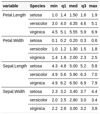
summarytools objects are not always compatible with packages focused on table formatting, such as formattable or kableExtra. However, tb() can be used as a “bridge”, an intermediary step turning freq() and descr() objects into simple tables that any package can work with. Here is an example using kableExtra:

library(kableExtra)
library(magrittr)
stby(iris, iris$Species, descr, stats = "fivenum") %>%
  tb(order = 3) %>%
  kable(format = "html", digits = 2) %>%
  collapse_rows(columns = 1, valign = "top")

6. Redirecting Output to Files

Using the file argument with print() or view(), we can write outputs to a file, be it html, Rmd, md, or just plain text (txt). The file extension is used to determine the type of content to write out.

view(iris_stats_by_species, file = "~/iris_stats_by_species.html")
view(iris_stats_by_species, file = "~/iris_stats_by_species.md")

A Note About PDF documents

There is no direct way to create a PDF file with summarytools. One option is to generate an html file and convert it to PDF using Pandoc or WK<html>TOpdf (the latter gives better results than Pandoc with dfSummary() output). Another option is to create an Rmd document using PDF as the output format, but with a caveat: displaying graphs with dfSummary() will cause vertical misalignment (we hope to resolve this issue in a future version).

6.1 Appending Output Files

The append argument allows adding content to existing files generated by summarytools. This is useful if we wish to include several statistical tables in a single file. It is a quick alternative to creating an Rmd document.

7. Global options

The following options can be set with st_options():

7.1 General Options

Option name	Default	Note
style (1)	“simple”	Set to “rmarkdown” in .Rmd documents
plain.ascii	TRUE	Set to FALSE in .Rmd documents
round.digits	2	Number of decimals to show
headings	TRUE	Formerly “omit.headings”
footnote	“default”	Customize or set to NA to omit
display.labels	TRUE	Show variable / data frame labels in headings
bootstrap.css (2)	TRUE	Include Bootstrap 4 CSS in html output files
custom.css	NA	Path to your own CSS file
escape.pipe	FALSE	Useful for some Pandoc conversions
char.split (3)	12	Threshold for line-wrapping in column headings
subtitle.emphasis	TRUE	Controls headings formatting
lang	“en”	Language (always 2-letter, lowercase)

1. Applies to freq(), ctable() and descr(); dfSummary() has its own style option (see section 7.2)
2. Set to FALSE in Shiny apps
3. Affects only html outputs for descr() and ctable()

7.2 Function-Specific Options

Option name	Default	Note
freq.cumul	TRUE	Display cumulative proportions in freq()
freq.totals	TRUE	Display totals row in freq()
freq.report.nas	TRUE	Display row and “valid” columns
freq.ignore.threshold (1)	25	Used to determine which vars to ignore
freq.silent	FALSE	Hide console messages
ctable.prop	“r”	Display row proportions by default
ctable.totals	TRUE	Show marginal totals
descr.stats	“all”	“fivenum”, “common” or vector of stats
descr.transpose	FALSE	Display stats in columns instead of rows
descr.silent	FALSE	Hide console messages
dfSummary.style	“multiline”	Can be set to “grid” as an alternative
dfSummary.varnumbers	TRUE	Show variable numbers in 1st col.
dfSummary.labels.col	TRUE	Show variable labels when present
dfSummary.graph.col	TRUE	Show graphs
dfSummary.valid.col	TRUE	Include the Valid column in the output
dfSummary.na.col	TRUE	Include the Missing column in the output
dfSummary.graph.magnif	1	Zoom factor for bar plots and histograms
dfSummary.silent	FALSE	Hide console messages
tmp.img.dir (2)	NA	Directory to store temporary images
use.x11 (3)	TRUE	Allow creation of Base64-encoded graphs

1. See section 2.1.4 for details
2. Applies to dfSummary() only
3. Set to FALSE in text-only environments

Examples

st_options()                      # Display all global options values
st_options('round.digits')        # Display the value of a specific option
st_options(style = 'rmarkdown',   # Set the value of one or several options
           footnote = NA)         # Turn off the footnote for all html output

8. Overriding Formatting Attributes

When a summarytools object is created, its formatting attributes are stored within it. However, we can override most of them when using print() or view().

8.1 Overriding Function-Specific Arguments

This table indicates what arguments can be used with print() or view() to override formatting attributes. Base R’s format() function arguments also apply, even though they are not reproduced here.

Argument	freq	ctable	descr	dfSummary
style	x	x	x	x
round.digits	x	x	x
plain.ascii	x	x	x	x
justify	x	x	x	x
headings	x	x	x	x
display.labels	x	x	x	x
varnumbers				x
labels.col				x
graph.col				x
valid.col				x
na.col				x
col.widths				x
totals	x	x
report.nas	x
display.type	x
missing	x
split.tables (*)	x	x	x	x
caption (*)	x	x	x	x

(*) These are pander options

8.2 Overriding Heading Contents

To change the information shown in the heading section, use the following arguments with print() or view():

Argument	freq	ctable	descr	dfSummary
Data.frame	x	x	x	x
Data.frame.label	x	x	x	x
Variable	x	x	x
Variable.label	x	x	x
Group	x	x	x	x
date	x	x	x	x
Weights	x		x
Data.type	x
Row.variable		x
Col.variable		x

Example

In the following example, we will create and display a freq() object, and then display it again, this time overriding three of its formatting attributes, as well as one heading attribute.

(age_stats <- freq(tobacco$age.gr)) 

## setting plain.ascii to FALSE

Frequencies

tobacco$age.gr
Type: Factor

	Freq	% Valid	% Valid Cum.	% Total	% Total Cum.
18-34	258	26.46	26.46	25.80	25.80
35-50	241	24.72	51.18	24.10	49.90
51-70	317	32.51	83.69	31.70	81.60
71 +	159	16.31	100.00	15.90	97.50
<NA>	25			2.50	100.00
Total	1000	100.00	100.00	100.00	100.00

print(age_stats, report.nas = FALSE, totals = FALSE, display.type = FALSE,
      Variable.label = "Age Group")

Frequencies

tobacco$age.gr
Label: Age Group

	Freq	%	% Cum.
18-34	258	26.46	26.46
35-50	241	24.72	51.18
51-70	317	32.51	83.69
71 +	159	16.31	100.00

8.3 Order of Priority for Parameters / Options

1. print() or view() parameters have precedence (overriding feature)
2. freq() / ctable() / descr() / dfSummary() parameters come second
3. Global options set with st_options() come third and act as default

9. Fine-Tuning Looks with CSS

When creating html reports, both Bootstrap’s CSS and summarytools.css are included by default. For greater control on the looks of html content, it is also possible to add class definitions in a custom CSS file.

Example

We need to use a very small font size for a simple html report containing a dfSummary(). For this, we create a .css file (with the name of our choosing) which contains the following class definition:

.tiny-text {
  font-size: 8px;
}

Then we use print()’s custom.css argument to specify to location of our newly created CSS file (results not shown):

print(dfSummary(tobacco), custom.css = 'path/to/custom.css', 
      table.classes = 'tiny-text', file = "tiny-tobacco-dfSummary.html")

10. Creating Shiny apps

To successfully include summarytools functions in Shiny apps,

• use html rendering
• set bootstrap.css = FALSE to avoid interacting with the app’s layout
• set headings = FALSE in case problems arise
• adjust graph sizes with print()’s graph.magnif parameter or with the dfSummary.graph.magnif global option
• if dfSummary() tables are too wide, omit a column or two (valid.col and varnumbers, for instance)
• if the results are still unsatisfactory, set column widths manually with print()’s col.widths parameter

Example (results not shown)

print(dfSummary(somedata, varnumbers = FALSE, valid.col = FALSE, 
                graph.magnif = 0.8), 
      method = 'render',
      headings = FALSE,
      bootstrap.css = FALSE)

11. Graphs in Markdown dfSummaries

When using dfSummary() in an Rmd document using markdown styling (as opposed to html rendering), three elements are needed in order to display the png graphs properly:

1 - plain.ascii must be set to FALSE
2 - style must be set to “grid”
3 - tmp.img.dir must be defined

Why the third element? Although R makes it really easy to create temporary files and directories, they do have long pathnames, especially on Windows. Unfortunately, Pandoc determines the final (rendered) column widths by counting characters in a cell, even if those characters are paths pointing to images.

At this time, there seems to be only one solution around this problem: cut down on characters in image paths. So instead of this:

+-----------+---------------------------------------------------------------------+---------+
| Variable  | Graph                                                               | Valid   |
+===========+=====================================================================+=========+
| gender\   | ![](C:/Users/johnny/AppData/Local/Temp/RtmpYRgetx/file5aa44d71.png) | 978\    |
| [factor]  |                                                                     | (97.8%) |
+----+---------------+------------------------------------------------------------+---------+

…we aim for this:

+---------------+----------------------+---------+
| Variable      | Graph                | Valid   |
+===============+======================+=========+
| gender\       | ![](/tmp/ds0001.png) | 978\    |
| [factor]      |                      | (97.8%) |
+---------------+----------------------+---------+

CRAN policies are really strict when it comes to writing content in the user directories, or anywhere outside R’s temporary zone (for good reasons). So the users need to set this location themselves, therefore consenting to having content written outside R’s predefined temporary zone.

On Mac OS and Linux, using “/tmp” makes a lot of sense: it’s a short path, and it’s self-cleaning. On Windows, there is no such convenient directory, so we need to pick one – be it absolute (“/tmp”) or relative (“img”, or simply “.”). Two things are to be kept in mind: it needs to be short (5 characters max) and it needs to be cleaned up manually.

12. Translations

Thanks to the R community’s efforts, the following languages can be used, in addition to English (default): French (fr), Portuguese (pt), Russian (ru), Spanish (es), and Turkish (tr).

To switch languages, simply use

st_options(lang = "fr")

All output from the core functions will now use that language:

freq(iris$Species)

## setting plain.ascii to FALSE

Tableau de fréquences

iris$Species
Type: Facteur

	Fréq.	% Valide	% Valide cum.	% Total	% Total cum.
setosa	50	33.33	33.33	33.33	33.33
versicolor	50	33.33	66.67	33.33	66.67
virginica	50	33.33	100.00	33.33	100.00
<NA>	0			0.00	100.00
Total	150	100.00	100.00	100.00	100.00

12.1 Non-UTF-8 Locales

On most Windows systems, it will be necessary to change the LC_CTYPE element of the locale settings if the character set is not included in the system’s default locale. For instance, in order to get good results with the Russian language in a “latin1” environment, we need to do the following:

Sys.setlocale("LC_CTYPE", "russian")
st_options(lang = 'ru')

Then to go back to default settings:

Sys.setlocale("LC_CTYPE", "")
st_options(lang = "en")

12.2 Defining and Using Custom Translations

Using the function use_custom_lang(), it is possible to add your own set of translations. To achieve this, get the csv template, customize the +/- 70 items, and call use_custom_lang(), giving it as sole argument the path to the edited csv template. Note that such custom translations will not persist across R sessions. This means that you should always have this csv file handy for future use.

12.3 Defining Specific Keywords

Sometimes, all you might want to do is change just a few keywords – for instance, you could prefer using “N” instead of “Freq” in the title row of freq() tables. For this, use define_keywords(). Calling this function without any arguments will bring up, on systems that support graphical devices (the vast majority, that is), an editable window allowing to modify only the desired item(s).

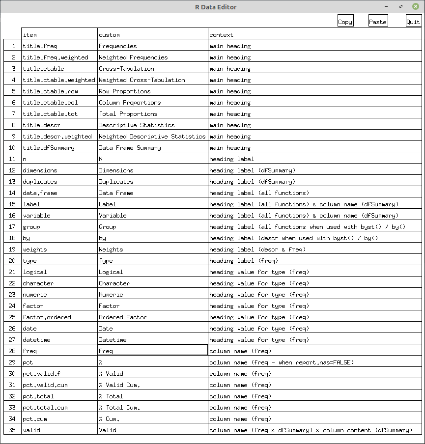
After closing the edit window, you will be able to export the resulting “custom language” into a csv file that you can reuse in the future by calling use_custom_lang().

It is also possible to programmatically define one or several keywords using define_keywords(). For instance:

define_keywords(freq = "N")

See ?define_keywords for more details.

13. Additional Software Installations

Required Software on Mac OS

Magick++

Open a terminal window and enter the following:

brew install [email protected]

If you do not have brew installed, simply enter this command in the terminal:

/usr/bin/ruby -e "$(curl -fsSL https://raw.githubusercontent.com/Homebrew/install/master/install)"

XQuartz

If you’re using Mac OS X version 10.8 (Mountain Lion) or more recent versions, you’ll need to download the .dmg image from xquartz.org and add it to your Applications folder.

Back to installation instructions

Required Software for Debian / Ubuntu / Linux Mint

Magick++
sudo apt install libmagick++-dev

Back to installation instructions

Required Software for Older Ubuntu Versions

This applies only if you are using Ubuntu Trusty (14.04) or Xenial (16.04).

Magick++

sudo add-apt-repository -y ppa:opencpu/imagemagick
sudo apt-get update
sudo apt-get install -y libmagick++-dev

Back to installation instructions

Required Software for Fedora / Red Had / CentOS

Magick++
sudo yum install ImageMagick-c++-devel

Back to installation instructions

Required Software for Solaris

Magick++

pkgadd -d http://get.opencsw.org/now
/opt/csw/bin/pkgutil -U
/opt/csw/bin/pkgutil -y -i imagemagick 
/usr/sbin/pkgchk -L CSWimagemagick

Back to installation instructions

14. Conclusion

The package comes with no guarantees. It is a work in progress and feedback is always welcome. Please open an issue on GitHub if you find a bug or wish to submit a feature request.

Stay Up to Date, and Get Involved!

For a preview of what’s coming in the next release, have a look at the development branch.

So far, I’ve worked a lot on my own on this project. Now I need your help to make it more of a collective effort. Check out the Wiki and don’t hesitate to post in the Discussions section.

15. Sponsors

A big thanks to people who made donations!

• Ashirwad Barnwal
• David Thomas
• Peter Nilsson
• Ross Dunne
• Igor Rubets

If you find summarytools useful and want to support its development, please consider making a small donation using the PayPal button.