NeuroPyxels: loading, processing and plotting Neuropixels data in python

NeuroPyxels (npyx) is a python library built for electrophysiologists using Neuropixels electrodes. This package stems from the need of a pythonist who really did not want to transition to MATLAB to work with Neuropixels: it features a suite of core utility functions for loading, processing and plotting Neuropixels data.

There isn't any better doc atm - post an issue if you have any question, or email Maxime Beau (PhD Hausser lab, UCL). You can also use the Neuropixels slack workgroup, channel #NeuroPyxels.

Documentation:

Npyx works in harmony with the data formatting employed by SpikeGLX and OpenEphys used in combination with Kilosort or SpyKING CIRCUS and Phy ([after conversion for the phy gui](https://spyking-circus.readthedocs.io/en/latest/GUI/launching.html, results stored in path/mydata/mydata.GUI)). Any dataset you can run phy on can also be analyzed with npyx, in essence.

Npyx is fast because it never computes the same thing twice - in the background, it saves most relevant outputs (spike trains, waveforms, correlograms...) at kilosort_dataset/npyxMemory, from where they are simply reloaded if called again. An important parameter controlling this behaviour is again (boolean), by default set to False: if True, the function will recompute the output rather than loading it from npyxMemory. This is important to be aware of this behaviour, as it can lead to mind boggling bugs. For instance, if you load the train of unit then re-spikesort your dataset, e.g. you split unit 56 in 504 and 505, the train of the old unit 56 will still exist at kilosort_dataset/npyxMemory and you will be able to load it even though the unit is gone!

Most npyx functions take at least one input: dp, which is the path to your Kilosort-phy dataset. You can find a full description of the structure of such datasets on phy documentation.

Other typical parameters are: verbose (whether to print a bunch of informative messages, useful when debugging), saveFig (boolean) and saveDir (whether to save the figure in saveDir for plotting functions).

Importantly, dp can also be the path to a merged dataset, generated with npyx.merge_datasets() - every function will run as smoothly on merged datasets as on any regular dataset. See below for more details.

More precisely, every function requires the files myrecording.ap.meta/myrecording.oebin (metadata from SpikeGLX/OpenEphys), params.py, spike_times.npy and spike_clusters.npy. If you have started spike sorting, cluster_groups.tsv will also be required obviously (will be created filled with 'unsorted' groups if none is found). Then particular functions will require particular files: loading waveforms with npyx.spk_wvf.wvf or extracting your sync channel with npyx.io.get_npix_sync require the raw data myrecording.ap.bin``myrecording.dat, npyx.spk_wvf.templates the files templates.npy and spike_templates.npy, and so on. This allows you to only transfer the strictly necassary files for your use case from a machine to the next: for instance, if you only want to make behavioural analysis of spike trains but do not care about the waveforms, you can run get_npix_sync on a first machine (which will generate a sync_chan folder containing extracted onsets/offsets from the sync channel(s)), then exclusively transfer the sync_chan folder along with spike_times.npy and spike_clusters.npy (all very light files) on another computer and analyze your data there seemlessly.

Directory structure

The dp parameter of all npyx functions must be the absolute path to myrecording below.

For SpikeGLX recordings:

myrecording/
  myrecording.ap.meta
  params.py
  spike_times.npy
  spike_clusters.npy
  cluster_groups.tsv # optional, if manually curated with phy
  myrecording.ap.bin # optional, if wanna plot waveforms

  # other kilosort/spyking circus outputs here

For Open-Ephys recordings:

myrecording/
  myrecording.oebin
  params.py
  spike_times.npy
  spike_clusters.npy
  cluster_groups.tsv # if manually curated with phy

  # other kilosort/spyking circus outputs here

  continuous/
    Neuropix-PXI-100.0/
      continuous.dat # optional, if wanna plot waveforms
    Neuropix-PXI-100.1/
      continuous.dat # optional, if want to plot LFP with plot_raw

  events/
    Neuropix-PXI-100.0/
      TTL_1/
        timestamps.npy # optional, if need to get synchronyzation channel to load with get_npix_sync e.g. to merge datasets

Example use cases are:

Load recording metadata

from npyx import *

dp = 'datapath/to/myrecording'

# load contents of .lf.meta and .ap.meta or .oebin files as python dictionnary.
# The metadata of the high and lowpass filtered files are in meta['highpass'] and meta['lowpass']
# Quite handy to get probe version, sampling frequency, recording length etc
meta = read_metadata(dp)

Load synchronization channel

from npyx.io import get_npix_sync # star import is sufficient, but I like explicit imports!

# If SpikeGLX: slow the first time, then super fast
onsets, offsets = get_npix_sync(dp)
# onsets/offsets are dictionnaries
# keys: ids of sync channel where a TTL was detected,
# values: times of up (onsets) or down (offsets) threshold crosses, in seconds.

Get good units from dataset

from npyx.gl import get_units
units = get_units(dp, quality='good')

Load spike times from unit u

from npyx.spk_t import trn
u=234
t = trn(dp, u) # gets all spikes from unit 234, in samples

Load waveforms from unit u

from npyx.io import read_spikeglx_meta
from npyx.spk_t import ids, trn
from npyx.spk_wvf import get_peak_chan, wvf, templates

# returns a random sample of 100 waveforms from unit 234, in uV, across 384 channels
waveforms = wvf(dp, u) # return array of shape (n_waves, n_samples, n_channels)=(100, 82, 384) by default
waveforms = wvf(dp, u, n_waveforms=1000, t_waveforms=90) # now 1000 random waveforms, 90 samples=3ms long

# Get the unit peak channel (channel with the biggest amplitude)
peak_chan = get_peak_chan(dp,u)
# extract the waveforms located on peak channel
w=waves[:,:,peak_chan]

# Extract waveforms of spikes occurring between
# 0-100s and 300-400s in the recording,
# because that's when your mouse sneezed
waveforms = wvf(dp, u, periods=[(0,100),(300,400)])

# alternatively, longer but more flexible:
fs=meta['highpass']['sampling_rate']
t=trn(dp,u)/fs # convert in s
# get ids of unit u: all spikes have a unique index in the dataset,
# which is their rank sorted by time (as in spike_times.npy)
u_ids = ids(dp,u)
ids=ids(dp,u)[(t>900)&(t<1000)]
mask = (t<100)|((t>300)&(t<400))
waves = wvf(dp, u, spike_ids=u_ids[mask])

# If you want to load the templates instead (faster and does not require binary file):
temp = templates(dp,u) # return array of shape (n_templates, 82, n_channels)

Compute auto/crosscorrelogram between 2 units

from npyx.corr import ccg, ccg_stack

# returns ccg between 234 and 92 with a binsize of 0.2 and a window of 80
c = ccg(dp, [234,92], cbin=0.2, cwin=80)

# Only using spikes from the first and third minutes of recording
c = ccg(dp, [234,92], cbin=0.2, cwin=80, periods=[(0,60), (120,180)])

# better, compute a big stack of crosscorrelograms with a given name
# The first time, CCGs will be computed in parallel using all the available CPU cores
# and it will be saved in the background and, reloadable instantaneously in the future
source_units = [1,2,3,4,5]
target_units = [6,7,8,9,10]
c_stack = ccg_stack(dp, source_units, target_units, 0.2, 80, name='my_relevant_ccg_stack')
c_stack = ccg_stack(dp, name='my_relevant_ccg_stack') # will work to reaload in the future

Plot waveform and crosscorrelogram of unit u

# all plotting functions return matplotlib figures
from npyx.plot import plot_wvf, get_peak_chan

u=234
# plot waveform, 2.8ms around templates center, on 16 channels around peak channel
# (the peak channel is found automatically, no need to worry about finding it)
fig = plot_wvf(dp, u, Nchannels=16, t_waveforms=2.8)

# But if you wished to get it, simply run
peakchannel = get_peak_chan(dp, u)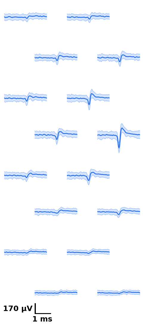

# plot ccg between 234 and 92
# as_grid also plot the autocorrelograms
fig = plot_ccg(dp, [u,92], cbin=0.2, cwin=80, as_grid=True)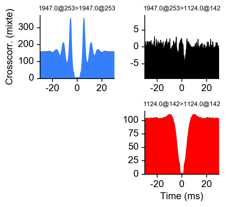

Plot chunk of raw data with overlaid units

units = [1,2,3,4,5,6]
channels = np.arange(70,250)
# raw data are whitened, high-pass filtered and median-subtracted by default - parameters are explicit below
plot_raw_units(dp, times=[0,0.130], units = units, channels = channels,
               colors=['orange', 'red', 'limegreen', 'darkgreen', 'cyan', 'navy'],
               lw=1.5, offset=450, figsize=(6,16), Nchan_plot=10,
               med_sub=1, whiten=1, hpfilt=1)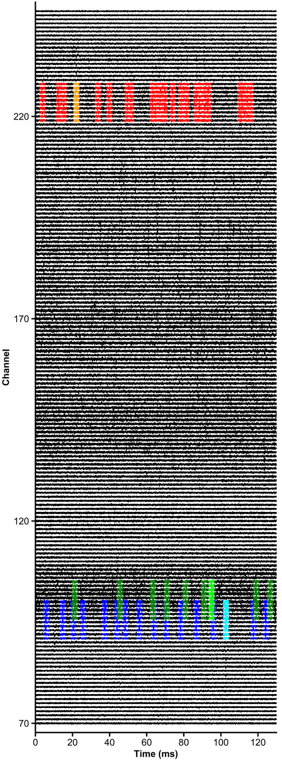

Plot peri-stimulus time histograms across neurons and conditions

# Explore responses of 3 neurons to 4 categories of events:
fs=30000 # Hz
units=[1,2,3]
trains=[trn(dp,u)/fs for u in units] # make list of trains of 3 units
trains_str=units # can give specific names to units here, show on the left of each row
events=[licks, sneezes, visual_stimuli, auditory_stimuli] # get events corresponding to 4 conditions
trains_str=['licking', 'sneezing', 'visual_stim', 'auditory_stim'] # can give specific names to events here, show above each column
events_col='batlow' # colormap from which the event colors will be drawn
fig=summary_psth(trains, trains_str, events, events_str, psthb=10, psthw=[-750,750],
                 zscore=0, bsl_subtract=False, bsl_window=[-3000,-750], convolve=True, gsd=2,
                 events_toplot=[0], events_col=events_col, trains_col_groups=trains_col_groups,
                 title=None, saveFig=0, saveDir='~/Downloads', _format='pdf',
                 figh=None, figratio=None, transpose=1,
                 as_heatmap=False,  vmin=None, center=None, vmax=None, cmap_str=None)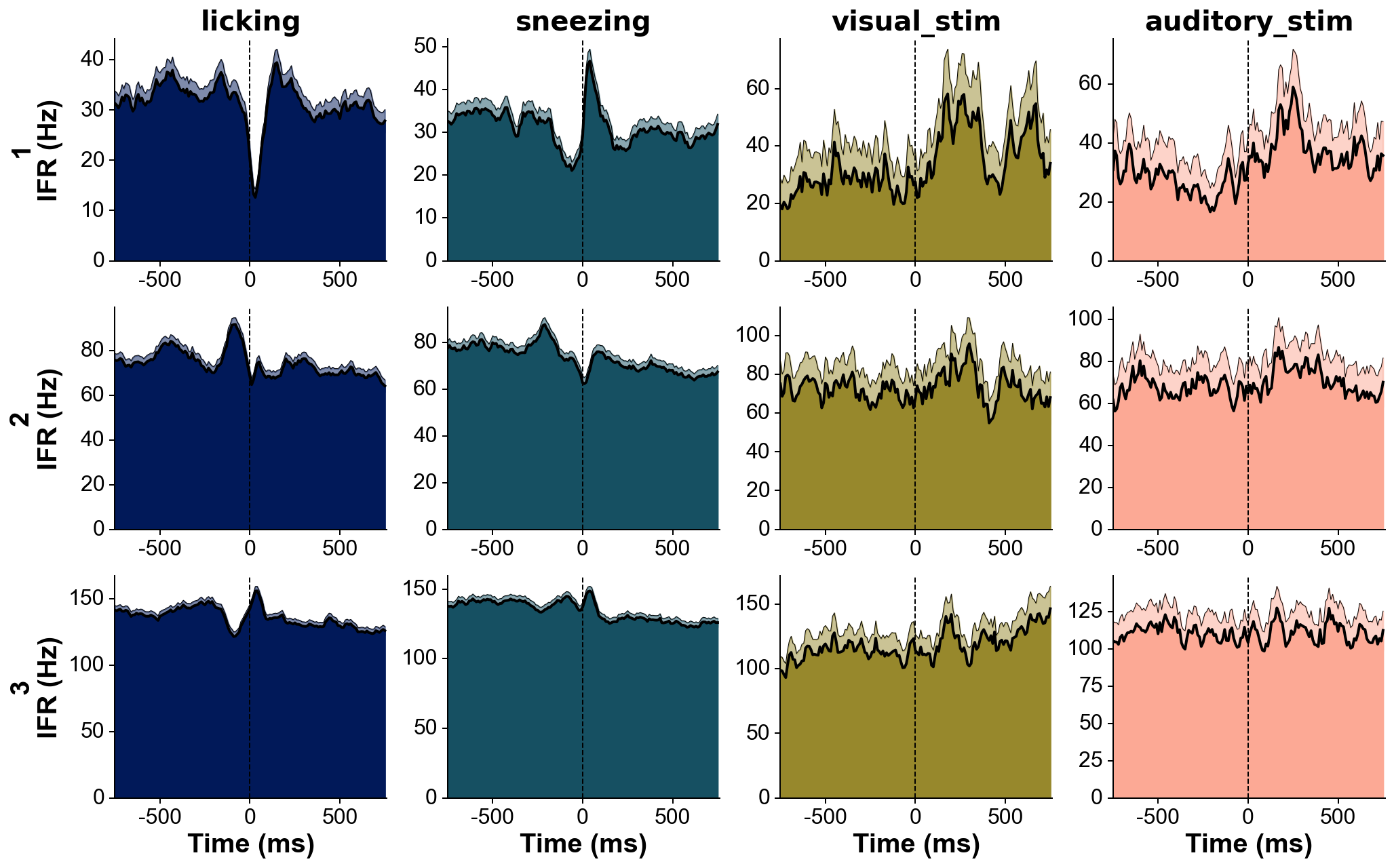

Merge datasets acquired on two probes simultaneously

# The three recordings need to include the same sync channel.
from npyx.merger import merge_datasets
dps = ['same_folder/lateralprobe_dataset',
       'same_folder/medialprobe_dataset',
       'same_folder/anteriorprobe_dataset']
probenames = ['lateral','medial','anterior']
dp_dict = {p:dp for p, dp in zip(dps, probenames)}

# This will merge the 3 datasets (only relevant information, not the raw data) in a new folder at
# dp_merged: same_folder/merged_lateralprobe_dataset_medialprobe_dataset_anteriorprobe_dataset
# where all npyx functions can smoothly run.
# The only difference is that units now need to be called as floats,
# of format u.x (u=unit id, x=dataset id [0-2]).
# lateralprobe, medial probe and anteriorprobe x will be respectively 0,1 and 2.
dp_merged, datasets_table = merge_datasets(dp_dic)


--- Merged data (from 2 dataset(s)) will be saved here: /same_folder/merged_lateralprobe_dataset_medialprobe_dataset_anteriorprobe_dataset.

--- Loading spike trains of 2 datasets...

sync channel extraction directory found: /same_folder/lateralprobe_dataset/sync_chan
Data found on sync channels:
chan 2 (201 events).
chan 4 (16 events).
chan 5 (175 events).
chan 6 (28447 events).
chan 7 (93609 events).
Which channel shall be used to synchronize probes? >>> 7

sync channel extraction directory found: /same_folder/medialprobe_dataset/sync_chan
Data found on sync channels:
chan 2 (201 events).
chan 4 (16 events).
chan 5 (175 events).
chan 6 (28447 events).
chan 7 (93609 events).
Which channel shall be used to synchronize probes? >>> 7

sync channel extraction directory found: /same_folder/anteriorprobe_dataset/sync_chan
Data found on sync channels:
chan 2 (201 events).
chan 4 (16 events).
chan 5 (175 events).
chan 6 (28194 events).
chan 7 (93609 events).
Which channel shall be used to synchronize probes? >>> 7

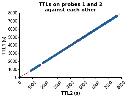
--- Aligning spike trains of 2 datasets...
More than 50 sync signals found - for performance reasons, sub-sampling to 50 homogenoeously spaced sync signals to align data.
50 sync events used for alignement - start-end drift of -3080.633ms

--- Merged spike_times and spike_clusters saved at /same_folder/merged_lateralprobe_dataset_medialprobe_dataset_anteriorprobe_dataset.

--> Merge successful! Use a float u.x in any npyx function to call unit u from dataset x:
- u.0 for dataset lateralprobe_dataset,
- u.1 for dataset medialprobe_dataset,
- u.2 for dataset anteriorprobe_dataset.

Now any npyx function runs on the merged dataset! Under the hood, it will create a merged_dataset_dataset1_dataset2/npyxMemory folder to save any data computed across dataframes, but will use the original dataset1/npyxMemory folder to save data related to this dataset exclusively (e.g. waveforms). Hence, there is no redundancy: space and time are saved.

This is also why it is primordial that you do not move your datatasets from their original paths after merging them - else, functions ran on merged_dataset1_dataset2 will not know where to go fetch the data! They refer to the paths in merged_dataset_dataset1_dataset2/datasets_table.csv. If you really need to, you can move your datasets but do not forget to edit this file accordingly.

# These will work!
t = trn(dp_merged, 92.1) # get spikes of unit 92 in dataset 1 i.e. medialprobe
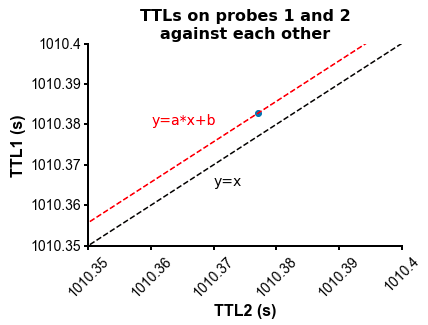
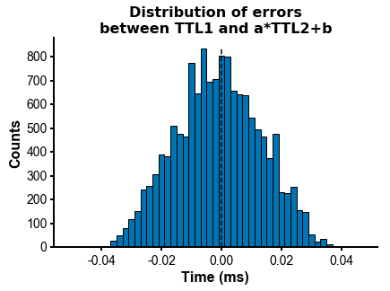
fig=plot_ccg(dp_merged,[10.0, 92.1, cbin=0.2, cwin=80]) # compute CCG between 2 units across datasets

PS - The spike times are aligned across datasets by modelling the drift between the clocks of the neuropixels headstages linearly: TTL probe 1 = a * TTL probe 1 + b (if a!=1, there is drift between the clocks), so spiketimes_probe2_aligned_to_probe1 = a * spiketimes_probe2 + b

Other npyx utility functions which could turn out useful

from npyx.utils import get_ncolors_cmap

# allows you to easily extract the (r,g,b) tuples from a matplotlib or crameri colormap
# to use them in other plots!
colors = get_ncolors_cmap('coolwarm', 10, plot=1)
colors = get_ncolors_cmap('viridis', 10, plot=1)
# in a jupyter notebook, will also plot he HTML colormap:

Installation:

Using a conda/virtualenv environment is very much advised, as pre-existing packages on a python installation might be incompatible with npyx and break your installation (typically leading to python -c 'import npyx' failing). Instructions here: manage conda environments

Npyx supports Python 3.7+.

as a user

from pip (normally up to date)

conda create -n my_env python=3.7
conda activate my_env
pip install npyx
python -c 'import npyx' # should not return any error
# If it does, (re)install any missing (conflictual) dependencies with pip (hopefully none!)
# and make sure that you are installing in a fresh environment.

from the remote repository (always up to date)

conda activate env_name
pip install git+https://github.com/Npix-routines/NeuroPyxels@master

as a superuser (recommended if plans to work on it/regularly pull upgrades)

Tip: in an ipython/jupyter session, use %load_ext autoreload then %autoreload to make your local edits active in your session without having to restart your kernel. Amazing for development.

conda activate my_env
cd path/to/save_dir # any directory where your code will be accessible by your editor and safe. NOT downloads folder.
git clone https://github.com/Npix-routines/NeuroPyxels
cd NeuroPyxels
pip install -e . --user # this will create an egg link to save_dir, which means that you do not need to reinstall the package each time you pull an udpate from github.
# alternatively python setup.py develop, but this doesn't handle dependencies as nicely as pip

and pull every now and then:

conda activate env_name
cd path/to/save_dir/NeuroPyxels
git pull
# And that's it, thanks to the egg link no need to reinstall the package!
# be careful though: this will break if you edited the package. If you wish to contribute, I advise you
# to either post issues and wait for me to fix your problem, or to get in touch with me and potentially
# create your own branch from where you will be able to gracefully merge your edits with the master branch
# after revision.

Known installation issues

cannot import numba.core hence cannot import npyx
Older versions of numba did not feature the .core submodule. You probably run a too old version of numba, vestigial from an old installation - make sure that you install npyx in a fresh conda environment si that happens to you, and eventually that numba is not installed in your root:
```
pip uninstall numba
conda activate my_env
pip uninstall numba
pip install numba
```

- core dumped when importing

This seems to be an issue related to PyQt5 required by opencv (opencv-python). Solution:

# activate npyx environment first
pip uninstall opencv-python
pip install opencv-python
# pip install other missing dependencies

Full log:

In [1]: from npyx import *
In [2]: QObject::moveToThread: Current thread (0x5622e1ea6800) is not the object's thread (0x5622e30e86f0).
Cannot move to target thread (0x5622e1ea6800)

qt.qpa.plugin: Could not load the Qt platform plugin "xcb" in "/home/maxime/miniconda3/envs/npyx/lib/python3.7/site-packages/cv2/qt/plugins" even though it was found.
This application failed to start because no Qt platform plugin could be initialized. Reinstalling the application may fix this problem.

Available platform plugins are: xcb, eglfs, linuxfb, minimal, minimalegl, offscreen, vnc, wayland-egl, wayland, wayland-xcomposite-egl, wayland-xcomposite-glx, webgl.

Aborted (core dumped)

Acknowledgement

If you enjoy this package and use it for your research, you can:

cite this github repo using its DOI: Beau, M., Lajko, A., Martínez, G., Häusser, M., & Kostadinov, D. (2021). NeuroPyxels: loading, processing and plotting Neuropixels data in python. Github, https://doi.org/10.5281/zenodo.5509776
star this repo using the top-right star button.

Cheers!

Developer cheatsheet

Useful link to create a python package from a git repository

Push local updates to github:

# ONLY ON DEDICATED BRANCH

cd path/to/save_dir/NeuroPyxels
git checkout DEDICATED_BRANCH_NAME # ++++++ IMPORTANT
git add.
git commit -m "commit details - try to be specific"
git push origin DEDICATED_BRANCH_NAME # ++++++ IMPORTANT

# Then pull request to master branch using the online github green button! Do not forget this last step, to allow the others repo to sync.

Push local updates to PyPI (Maxime)

First change the version in ./setup.py in a text editor

setup(name='npyx',
      version='1.0',... # change to 1.1, 1.1.1...

Then delete the old distribution files before re-generating them for the new version using twine:

rm -r ./dist
rm -r ./build
rm -r ./npyx.egg-info
python setup.py sdist bdist_wheel # this will generate version 1.1 wheel without overwriting version 1.0 wheel in ./dist

Before pushing them to PyPI (older versions are saved online!)

twine upload dist/*

Uploading distributions to https://upload.pypi.org/legacy/
Enter your username: your-username
Enter your password: ****
Uploading npyx-1.1-py3-none-any.whl
100%|████████████████████████████████████████████████████████| 156k/156k [00:01<00:00, 96.8kB/s]
Uploading npyx-1.1.tar.gz
100%|█████████████████████████████████████████████████████████| 150k/150k [00:01<00:00, 142kB/s]

Cheap and reliable Node.js hosting starts at $3/month, and $1/month static HTML hosting

m-beau / NeuroPyxels

Programming Languages

Labels

Projects that are alternatives of or similar to NeuroPyxels