Fast non-linear gravity inversion in spherical coordinates with application to the South American Moho

by Leonardo Uieda and Valéria C. F. Barbosa

Published in the Geophysical Journal International: doi:10.1093/gji/ggw390

Click on this button to run the code online:

An archived snapshot of this repository is available on figshare at doi:10.6084/m9.figshare.3987267 (the manuscript LaTeX sources are not included).

A PDF of the article is available at leouieda.com/papers/paper-moho-inversion-tesseroids-2016.html

Contents:

• Python source code that implements the Moho inversion method proposed in the paper (see code/mohoinv.py). The modeling code uses the open-source geophysics library Fatiando a Terra.
• Data files required to produce all results and figures presented in the paper.
• Source code in Jupyter notebooks that produce all results and figures (the .ipynb files in code). You can view static (not executable) versions of these notebooks through the links provided in code/README.md.
• All figures in EPS format for the paper.
• Latex source to produce the manuscript (not included in the figshare archive).
• The estimated Moho depth model for South America, available in the file model/south-american-moho.txt in ASCII xyz format (download the file).

The main result from this publication is the gravity-derived Moho depth model for South America and the differences between it and seismological estimates of Assumpção et al. (2013):

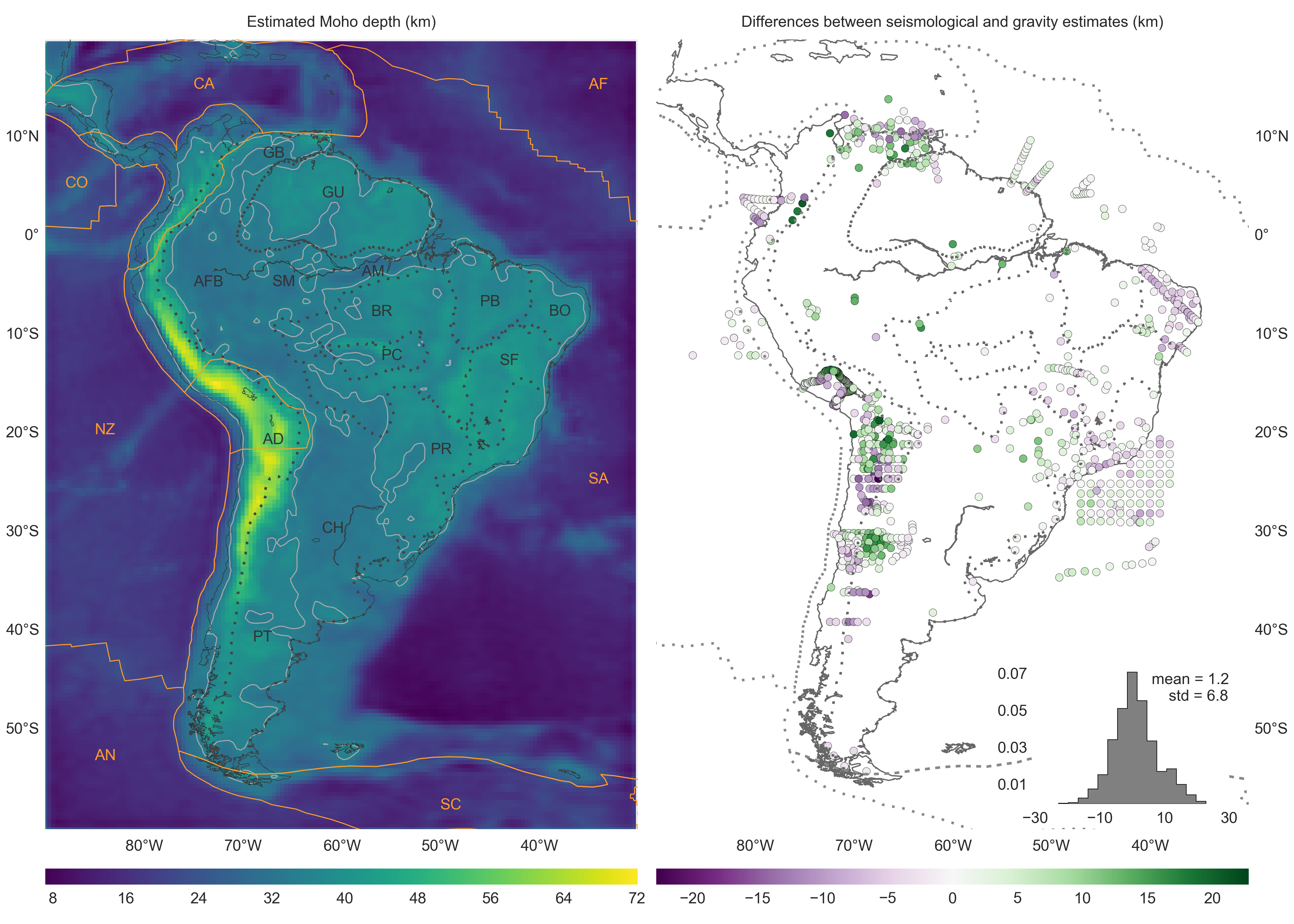
Dotted lines represent the boundaries between major geologic provinces. AD: Andean Province, AFB: Andean foreland basins, AM: Amazonas Basin, BR: Brazilian Shield, BO: Borborema province, CH: Chaco Basin, GB: Guyana Basin, GU: Guyana Shield, PB: Parnaíba Basin, PC: Parecis Basin, PR: Paraná Basin, PT: Patagonia province, SF: São Francisco Craton, SM: Solimões Basin. Solid orange lines mark the limits of the main lithospheric plates. AF: Africa Plate, AN: Antarctica Plate, CA: Caribbean Plate, CO: Cocos Plate, SA: South America Plate, SC: Scotia Plate, NZ: Nazca Plate. The solid light grey line is the 35 km Moho depth contour.

Abstract

Estimating the relief of the Moho from gravity data is a computationally intensive non-linear inverse problem. What is more, the modeling must take the Earths curvature into account when the study area is of regional scale or greater. We present a regularized non-linear gravity inversion method that has a low computational footprint and employs a spherical Earth approximation. To achieve this, we combine the highly efficient Bott's method with smoothness regularization and a discretization of the anomalous Moho into tesseroids (spherical prisms). The computational efficiency of our method is attained by harnessing the fact that all matrices involved are sparse. The inversion results are controlled by three hyper-parameters: the regularization parameter, the anomalous Moho density-contrast, and the reference Moho depth. We estimate the regularization parameter using the method of hold-out cross-validation. Additionally, we estimate the density-contrast and the reference depth using knowledge of the Moho depth at certain points. We apply the proposed method to estimate the Moho depth for the South American continent using satellite gravity data and seismological data. The final Moho model is in accordance with previous gravity-derived models and seismological data. The misfit to the gravity and seismological data is worse in the Andes and best in oceanic areas, central Brazil and Patagonia, and along the Atlantic coast. Similarly to previous results, the model suggests a thinner crust of 30-35 km under the Andean foreland basins. Discrepancies with the seismological data are greatest in the Guyana Shield, the central Solimões and Amazonas Basins, the Paraná Basin, and the Borborema province. These differences suggest the existence of crustal or mantle density anomalies that were unaccounted for during gravity data processing.

Reproducing the results

Executing the code online

You can run the Jupyter notebooks online without installing anything through the free Binder webservice:

mybinder.org/repo/pinga-lab/paper-moho-inversion-tesseroids

Start by navigating to the code folder and choose a notebook to execute. Beware that the CRUST1.0 and South American Moho notebooks will probably not be able to run on Binder because they take too long (a few days). If you want to try out the method start with the code/synthetic-simple.ipynb notebook or see how the figures for the paper are generated in the code/paper-figures.ipynb notebook. Tip: use Shift + Enter to execute a code cell.

If you want to run the full inversion on your machine, follow the steps below.

Running things on your machine

First, download a copy of all files in this repository:

• Download a zip archive

• Or clone the git repository:

    git clone https://github.com/pinga-lab/paper-moho-inversion-tesseroids.git
  

Setting up your environment

You'll need a working Python 2.7 environment with all the standard scientific packages installed (numpy, scipy, matplotlib, etc). The easiest (and recommended) way to get this is to download and install the Anaconda Python distribution. Make sure you get the Python 2.7 version.

All required dependencies are specified in the environmet.yml file. The exact versions of every dependency are also specified in the conda-*.lock files. The lock files can be used to create an exact version of the environment used in the paper for Linux, Mac, and Windows.

You can use conda package manager (included in Anaconda) to create a virtual environment with all the required packages installed. First, unzip the contents of this repository (if you've downloaded the zip file) and cd into the root of the repository (where environment.yml and the conda-*.lock files are located). Next, run the following command in a terminal (substituting the appropriate lock file for your operating system):

conda create -n moho --file conda-linux-64.lock

This will create the virtual environment based on the specifications in environment.yml and install all required dependencies. To activate the conda environment, run

source activate moho

or, if you're on Windows,

activate moho

This will enable the environment for your current terminal session.

Running the inversions and generating figures

The inversion and figure generation are all run inside Jupyter notebooks. To execute them, you must first start the notebook server by going into the repository folder and running (make sure you have the conda environment enabled first):

jupyter notebook

This will start the server and open your default web browser to the Jupyter console interface. In the page, go into the code folder and select the notebook that you wish to view/run.

Here what a notebook looks like running in Firefox:

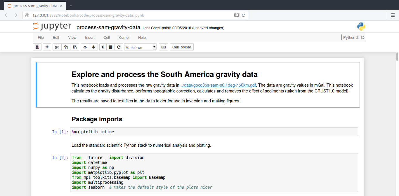
The notebook is divided cells (some have text while other have code). Each can be executed using Shift + Enter. Executing text cells does nothing and executing code cells runs the code and produces it's output. To execute the whole notebook, run all cells in order.

All results figures in the paper are generated by the code/paper-figures.ipynb notebook.

License

All source code is made available under a BSD 3-clause license. You can freely use and modify the code, without warranty, so long as you provide attribution to the authors. See LICENSE.md for the full license text.

The model results in file model/south-american-moho.txt are available under the Creative Commons Attribution 4.0 License (CC-BY).

The manuscript text is not open source. The authors reserve the rights to the article content, which has been accepted for publication in the Geophysical Journal International.