Pilotguru
- What?
- Current status
- Requirements
- Recording data
- Postprocessing - motion inference from data
- Processing detals and output data format
What?
Pilotguru is a project aiming to make it possible, with just a smartphone and zero hardware work, to gather all the necessary data to train your own computer vision based car autopilot/ADAS:
- With pilotguru recorder, use a smartphone as a dashcam to record a ride (video + GPS data + accelerometer + gyroscope).
- With pilotguru, annotate frames of the recording with horizontal angular velocity (for steering) and
forward speed (for acceleration and braking).
- Repeat 1-2 until you have enough data.
- Train a machine learning model to control a car based on your garthered data. Pick an existing good one or build your own.
- If you are really feeling adventurous, intergrate your model with openpilot. You will have to have a compatible car and get some hardware to get it to actually control the car. Make sure to comply with the local laws, you assume all the responsibility for consequences, this software comes with no guarantees, yada yada yada.
- Self-driving cars solved! Enjoy ;)
Current status
- Android app to record timestamped video, GPS, accelerometer and gyroscope data: [Play Store], [source code].
- Forward velocity and steering angular velocity inferred from inertial measurements (accelerometer + gyroscope) and GPS data: [how to run], [demo].
Requirements
Data recording: Android phone with Marshmallow (6.0) or more recent version.
Data processing: Linux, docker. Everything runs in a docker image, the necessary dependencies will be pulled when you build the image.
Recording data
-
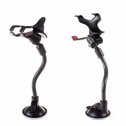
Get a windshield/dash phone mount for your car. We will use the phone motion to capture the motion of the car, so the less flex and wobble in the mount, the better. Long-armed mounts like this are probaby not very good for our use. Something like this would be better. Make sure the phone camera has a good view out of the windshield.
-
After you have secured the phone in the windshield mount, press the record button and go for a ride. Remember to not adjust the phone in the mount while data is recorded. We assume the motion of the phone to match the motion of the car, so moving the phone relative to the car will make the data useless.
-
Once you stop the recording, the results are saved to a new directory on the phone, named like
PilotGuru/2017_04_21-14_05_32(coresponding to the time of recording start).The directory will contain (see here for the details on data formats)
video.mp4- the video stream.frames.json- video frames timestamps.accelerations.json- raw accelerometer readings.rotations.json- raw gyroscope readings.locations.json- GPS data (locations and velocities).
Copy the whole directory to your computer for postprocessing.
Postprocessing - motion inference from data
Installation
- Clone this repo.
git clone https://github.com/waiwnf/pilotguru.git cd pilotguru - Build the docker image (this will take a while).
./build-docker.sh - Build everything (inside a docker container).
./run-docker.sh
mkdir build
cd build
cmake ..
make -j
Everything below should be run from inside the docker container (i.e. after executing ./run-docker.sh from pilotguru root directory).
Vehicle motion inference from GPS and IMU data
Velocity data comes from two separate sources with very distinct characteristics:
- GPS readings.
- Pros: Distinct measurements have independent errors. This is an extremely valuable property, it means the errors do not compound over time.
- Cons: Relatively coarse-grained, both in time (typically comes at around 1 update per second) and space (can be off by a few meters). May not be able to capture well important events like starting hard braking when an obstacle suddenly appears.
- Inertial measurement unit (IMU) readings: accelerometer and gyroscope.
- Pros: Can be very fine-grained (e.g. up to 500Hz measurement rate on a Nexus 5X), so very promising for precise annotation on video frames level.
- Cons: Inertial measurements use the immediate previous state (pose + velocity) of the device as a reference point. To get the device trajectory one needs to integrate the accelerations over time, so the measurement errors accumulate over time: acceleration measurement error on step 1 "pollutes" velocity estimates on each subsequent step. Even worse is the travel distance computation, where we need to integrate accelerations twice and the errors grow quadratically with time.
We will fuse the two data sources to combine the advantages and cancel out the drawbacks. GPS data will provide "anchor points" and let us eliminate most of the compounding errors from integrating the IMU data.
The fusion is done by fit_motion binary with JSON files produced by pilotguru recorder as inputs:
    ./fit_motion \
        --rotations_json /path/to/rotations.json \
        --accelerations_json /path/to/accelerations.json \
        --locations_json /path/to/locations.json \
        --velocities_out_json /path/to/output/velocities.json \
        --steering_out_json /path/to/output/steering.json
The outputs are two files:
velocities.jsonwith inferred vehicle velocities for every IMU measurement. See here for computation details.steering.jsonwith angular velocities in the inferred horizontal (i.e. road surface) plane, corresponding to car steering. See here for computation details.
Visualize results
Render a video with steering and velocity infdormation overlayed with the original input video:
./render_motion \
    --in_video /path/to/video.mp4 \
    --frames_json /path/to/frames.json \
    --velocities_json /path/to/output/velocities.json \
    --steering_json /path/to/output/steering.json \
    --steering_wheel /opt/pilotguru/img/steering_wheel_image.jpg \
    --out_video /path/to/output/rendered-motion.mp4
This will produce a video like this with a rotating steering wheel and a digital speedometer tiled next to the original ride recording. The steering wheel rotation should closely match the car steering.
Caveat: the steering wheel rotation in the rendering is somewhat misleading: it is proportional to the angular velocity of the car, so for turns at slow speed the rendered steering wheel will rotate less than the real one in the car, and vice versa for high speed.
Processing detals and output data format
Forward velocity
We aim to combine GPS data (coarse grained, but no systematic drift over time) with inertial measurements unit data (fine-grained, but prone to systematic drift) to combine the advantages of the two data sources and get fine-grained precise velocity data.
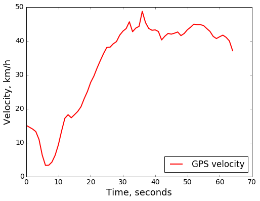
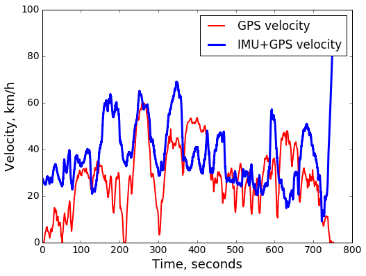
Before diving into details, notice that GPS data by itself is actually quite precise, at least with a decent view of clear sky. Here is an example track:
There are a couple of areas where we can count on improving the accuracy somewhat:
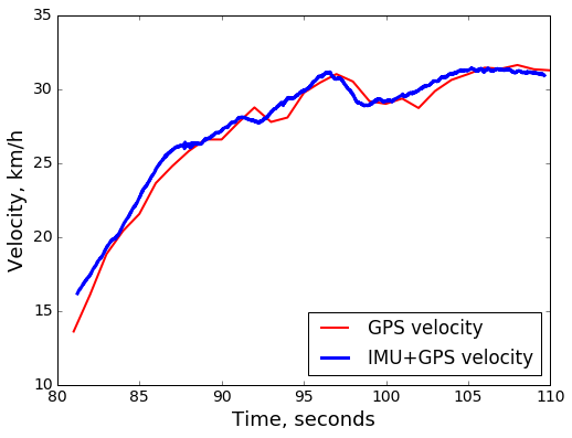
- Velocity jumps between the 30 second and 40 second marks are suspicious.
- GPS-derived velocity by its nature lags behind the true velocity changes, since we need to wait until the next measurement to compute the estimated velocity over the ~1 second interval. So during significant acceleration or braking there may be substantial difference between the GPS reported velocity (averaged over the past 1 second) and the true instantaneous velocity.
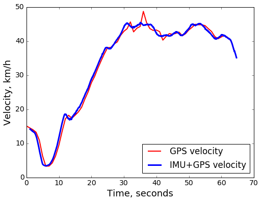
After incorporating the IMU data, we indeed see improvements on both counts. Noisy jumps are smoothed out and sustained sharp velocity changes are registered earlier:
IMU processing challenges
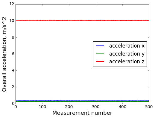
Some of the accelerometer processing challenges can be seen by simply looking at the raw accelerometer sensor readings from a phone lying flat on the table:
One can note that
- Gravity is not subtracted away by the sensor automatically. Theoretically Android has logic to do that on the OS level, but it requires extra calibration by the user (which I am trying to avoid in the overall process if at all possible) and did not seem to be precise enough in my experience.
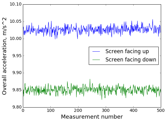
- Overall acceleration magnitude is quite far from 1g = 9.81 m/s^2. This suggests additional bias in the sensor.
Significant sensor bias is confirmed by comparing the readings from the phone laying screen up and screen down:
Calibration problem formulation
Formalizing the above section, define the calibration problem for the IMU unit to find the optimal
g: accelerometer bias in the fixed reference frame (this is roughly gravity).h: accelerometer bias in the device-local reference frame (this is the bias introduced by the sensor itself).v0: Initial velocity (3D) at the beginning of the recording sequence to support recordings that start when the car is already in motion.
The optimization objective is helpfully provided by the coarse grained "mostly correct" GPS data: for every interval between two neighbnoring GPS measurements we will aim to match the travelled distance of the calibrated IMU trajectory with the distance from GPS data. Using L2 loss function, we get
where
iis the index of a GPS measurement.k_i ... k_(i+1)are the range of indices for IMU measurements that fall in time between GPS measurementsiandi+1. is the time of the
 j-th IMU measurement.
Next, unroll the integrated IMU velocity in terms of measured raw accelerations and calibration parameters. Denote  and
and  .
.
where R_j is the rotation matrix from the device-local reference frame to the fixed reference time at time step j. The rotation matrix can itself be computed by integrating the rotational velocities measured by the gyroscope. Denoting W to be the derivative of the rotation matrix coming from the gyroscope, in the first approximation we have
In reality, this linear approximation is not used. The gyroscope does not report the derivative W directly. Instead it reports angular velocities around the 3 device axes, from which (and time duration) it is possible to compute the rotation matrix exactly. It is interesting to look at the first-order approximation though to highlight the linear time dependence.
Summing everything up, we arrive at the final calibration objective:
Despite looking a bit hairy, it is actually a nice quadratic objective with derivatives that are straightforward to compute analytically. It can thus be optimized efficiently with L-BFGS, which is a standard limited-memory second order optimization algorithm, to find the optimal calibration parameters g, h and v0.
Local calibration
... aka error accumulation strikes back.
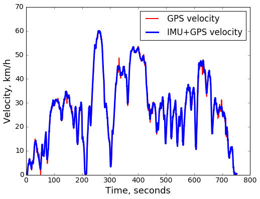
Though the IMU calibration objective captures several important sources of trajectory integration errors, there are also aspects that it ignores. For example both unavoidable white noise in measurements and systematic gyroscope measurement bias are completely ignored. IMU integration errors compound at quadratic rate (as a function of time). Hence for long (more than a couple of minutes) recordings, even after calibration the reconstructed IMU velocities may be totally off, such as in this example (the IMU+GPS velocity is the best match with respect to the calibration objective):
On the other hand, for shorter durations (~ 1 minute), calibrated IMU data yields a well matching result:
That calibration works well on shorter time ranges suggests an easy workaround. Instead of trying to capture all possible sources of integration error and fit the corresponding calibration parameters in the model, we slide a window of moderate duration (40 seconds by default) over the recorded time series, and each time calibrate the IMU only within that sliding window. The resulting estimated velocity for each timestamp is the average of values for that timestamp over all sliding windows containing that time. The result is a trajectory that at each point closely follows the dynamic measured by the IMU and at the same time "sheds" the accumulating integration error by re-anchoring itself to the GPS measurements:
Inferred velocity data format
Output data is a JSON file with timestamped absolute velocity magnitudes (no direction information) in m/s:
{
  "velocities": [
    {
      "speed_m_s": 0.031
      "time_usec": 567751960167
    },
    {
      "speed_m_s": 0.030
      "time_usec": 567751962707
    },
    ...
  ]
}
Steering angle
Computation details
Unlike accelerometer, gyroscope data does not suffer from noticeable systematic bias on our timescales (tens of minutes). The main problem with the raw data is that
- There is no notion of the road surface plane.
- The vehicle can rotate around all 3 possible axes: in addition to vertical axis (yaw, steering), rotation is possible around both the lateral axis (pitch, e.g. when transitioning from uphill to downhill road, or coming across a speed bump) and around longitudinal axis (roll, e.g. when driving into a pothole on one side of the car).
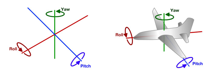
So the goal with rotation data is to infer the vertical axis in the vehicle reference frame. Then projecting instantaneous rotational velocity (in 3D) on the vertical axis yields the steering related rotation. Fortunately, the Earth locally is almost flat, so both pitch and roll rotations magnitude will be much smaller than steering-related yaw rotation. So we can well approximate the vertical axis as the one around which most of the rotation happens.
Mathematically, a convenient way to capture the main principal rotation axis is to employ a quaternion rotation representation. Rotation around an axis with direction (ax,ay,az) (normalized to unit length) through an angle a can be represented as a quaternion (4D vector):
q == (
  qx = ax * sin(a/2),
  qy = ay * sin(a/2),
  qz = az * sin(a/2),
  qw = sqrt(1 - x^2 - y^2 - z^2)
)
One can see that the first 3 components of the rotation quaternion capture both the direction and magnitude of rotation. We can then take all the recorded rotations (recorded in the moving device reference frame), integrated over intervals on the order of 1 second to reduce noise, ans apply principal components analysis to the first 3 quaternion components (qx, qy, qz). The first principal component of the result will be the axis (in the moving device reference frame) that captures most of the rotation overall. This first principal component is assumed to be the vertical axis of the vehicle. We then simply project all the rotations onto that axis to get the steering (yaw) rotation component.
Steering angular velocity data format
Output data is a JSON file with timestamped angular velocity around the inferred vehicle vertical axis:
{
  "steering": [
    {
      "angular_velocity": 0.02
      "time_usec": 567751960134
    },
    {
      "angular_velocity": -0.01
      "time_usec": 567751962709
    },
    ...
  ]
}