QGIS outdoor map

A simple map for outdoor activities as QGIS project for manual editing, printing, layouting, etc.

QGIS enables you to create PDF or image exports which then can be printed:

Example online maps

Take a look at these examples:

• Thüringer Wald (thuringian forest) (as of 04-2022; JPG; DPI 96)
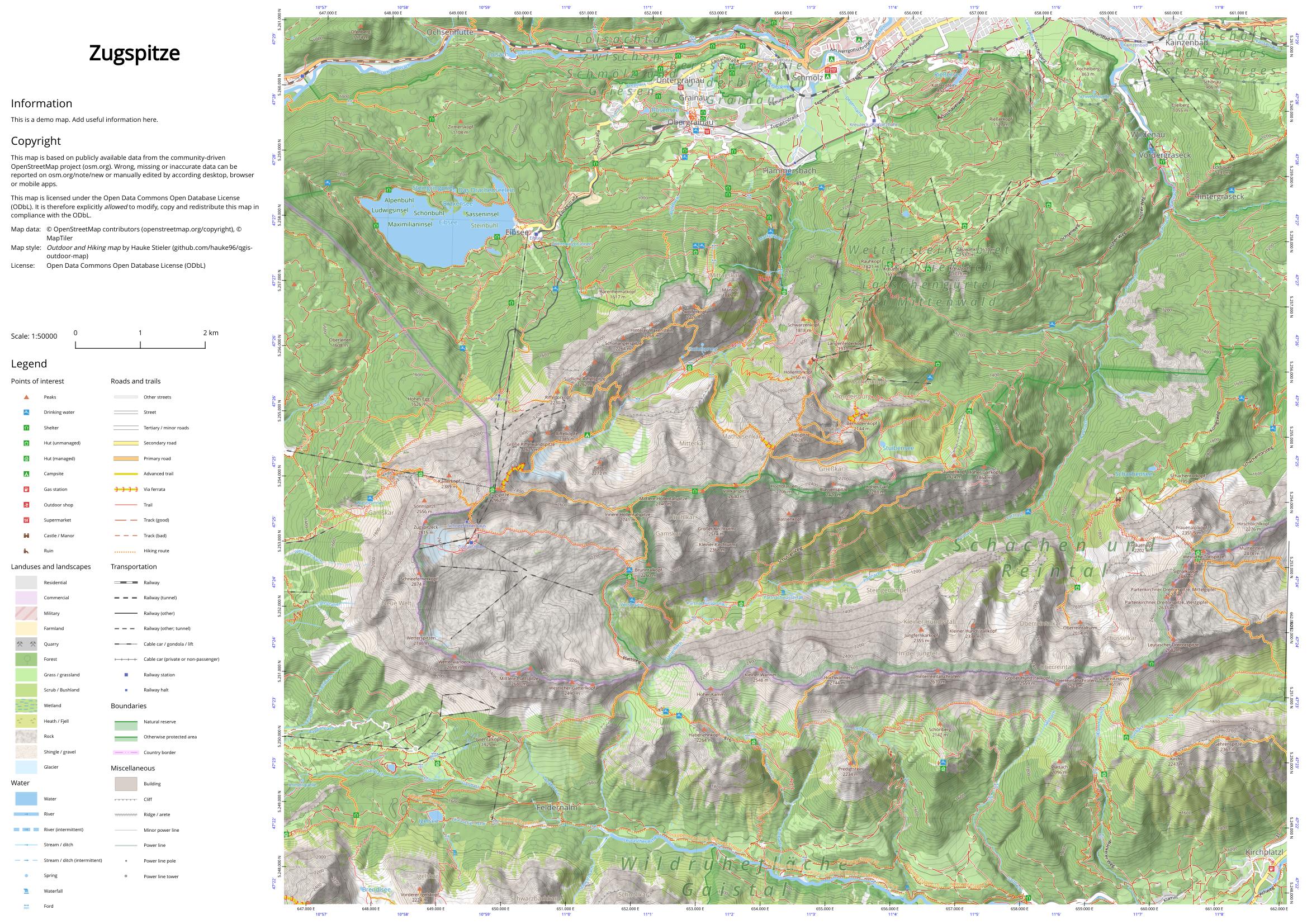
• Zugspitze / Castle Neuschwanstein (as of 11-2022; PNG; DPI 150)

How to use

1. Make sure you have a postgres database running (see section "Docker Setup" to start the database as a docker container)
2. Import data into the database (see "Fill database")
3. Read the "QGIS setup" section
4. Load the map.qgs project file
5. Take a look at the "Render map" section on how to render the map to PDF/PNG

Docker Setup

This QGIS-project expects a PostGIS database with the credentials postgres and secret. To make things easier there's a docker-compose file to start everything within a couple of seconds.

Setup

This folder contains the following docker related files:

• docker-compose.yml: Core docker file, needed to tell docker what to start. This also contains credentials for the database.
• init.sh: Simple script to fill a running database.
  • init.sh file.pbf will remove the current data and just import file.pbf
  • init.sh --append file.pbf will append the data from file.pbf to the current database
• .pgpass: Contains the credentials for the database. This is used by the init.sh script to be able to log into the database without user interactions.
• map.qgs: The actual QGIS project
• data/import-layout-data.sh: Downloads old/missing data and imports it specifically for a given layout.

Start

To start everything using docker, do the following:

1. Execute the following command within this folder: docker-compose up --build. This starts the docker container with an empty postgres database and postgis plugin.

That's it, your database is now running and can be filled with data.

Fill database

Make sure the database is running. Now we can add some data to it:

1. Download data

• When importing for a specific layout: Go into the data folder and execute the import-layout-data.sh script with the layout name as parameter (e.g. a2-thueringer-wald).
• When importing arbitrary data: Get a PBF-file (e.g. downloading from Geofabrik) of the area you want to work on. Downloading large areas just make things slow, so download only the stuff you need.

2. Fill the database with init.sh your-data.pbf. Caution: This removes the existing content of the database! Use --append to just append to existing data without wiping the database.

Combine multiple Extracts

Sometimes a region is across multiple Geofabrik extracts (e.g. your region covers Lower Saxony and Hamburg), in this case you have to combine multiple PBF-files into one.

The script ./data/import-layout-data.sh does that, so take a look at its source code.

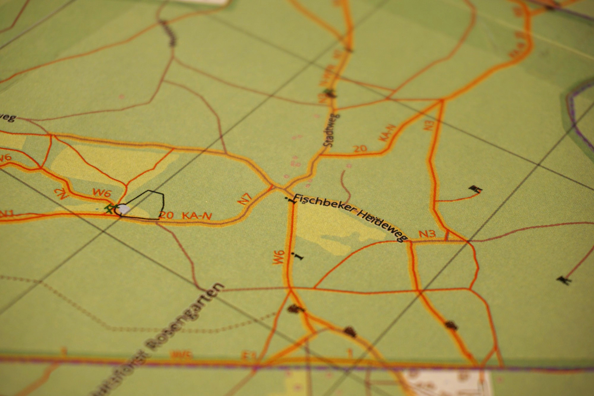
Example: Fischbek

The Hamburg-extract from Geofabrik does not contain the whole area of Fischbeker Heide, so we have to combine it with the Lower Saxony extract:

• Download Hamburg and Lower Saxony extracts
• Cutout irrelevant stuff from Lower Saxony: osmium extract -b 9.7685,53.4721,9.973,53.3978 niedersachsen-latest.osm.pbf --overwrite -o niedersachsen-latest-cutout.osm.pbf
• Merge them: osmium merge hamburg-latest.osm.pbf niedersachsen-latest-cutout.osm.pbf --overwrite -o hh-nds.pbf
• Import it: ./init.sh hh-nds.pbf

Update data

Updating data works just like in the "Fill database" step.

1. Download latest PBF file
2. Import into existing (filled or empty) database with init.sh your-data.pbf. Caution: This removes the existing content of the database! If you want to append data to the existing database use the --append flag (s. above).

This also works while QGIS is running.

Append data to database

Just use the --append parameter for the init.sh script: init.sh --append file.pbf

Hillshading & contour lines

Use the tutorial in this repo to create your own hillshade and contour lines files. This project has two layers (one for hillshading and one for contour lines), you just need to change the source to a lokcal .tif (for hillshading) or .gpkg (for contours) file.

For hillshading, there's also a public service provided by ESRI but the contours must be created locally (until I find a suitable public layer for that).

QGIS setup

1. Make sure you use the latest QGIS version (as of 15th December 3.22)
2. If you want to modify the project and create a pull-request:
3. Install the extension "Trackable QGIS Project" (this orders the XML attributes in the project file alphabetically so that the file is better trackable by git)
4. Collapse all layers before committing (just to keep the project clean)

Render map

Make sure the project is loaded in QGIS and that you have the data loaded into your database.

1. Create a layout or change an existing one
2. Add the OSM attribution if you use OSM data
3. Use the normal QGIS mechanisms to export the layout to PDF, PNG, ...

Render via Terminal/CLI

1. Make sure you created your layout in QGIS
2. Use the render-layout.py script to render a single layout (ude render-layout.py --help for more information)

Render all pre-defined layouts

There are some pre-defined layouts (such as a2-fischbeker-heide) wich legend, scale bar, attribution and everything. Calling the script render-all.sh renders them all as PDF and PNG files, no parameter needed.

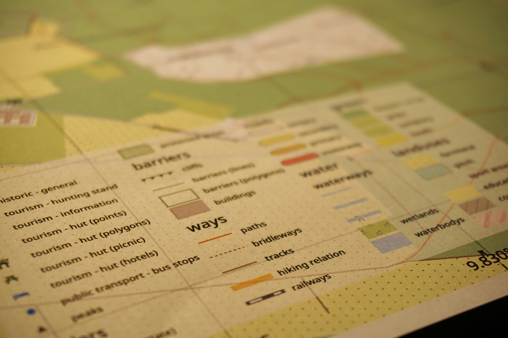
Style guideline

Some guidelines how the map style has been developed

Simplicity

Avoid unnecessary details and too many object. For example there's no styling difference between several road types like service, residential oder unclassified.

Font sizes

Normal font size is 6pt and used for streets and small places (e.g. place=square). But there are situations for larger fonts:

6pt

• streets
• hotels, guest houses

8pt

• small places
• grass areas
• forest
• heath
• hamlet, square, locality
• landuses (education, military, etc.)
• train stations

10pt

• village, city quarter
• protected area

12pt

• suburb

14pt

• city

Colors

The colors come from the material design colore palette and objects of the same kind have usually the same saturation and just different color tones. For example do all normal roads have the 200 saturation and all tunnel roads the 100 saturation.

Exceptions:

• Tidalflat areas have #bbd2dc (which is the "Blue Grey 100" color but with 20% saturation and 90% brightness instead)
• Pitches have #bde2d2 (the middle between "Green 100" and "Teal 100")
• Sport centres have #e8f5e9 ("Green 50" but with saturation of 10 instead of 5)
• Tracks have the #a1887f color but with 20° hue and 75% saturation (resulting in #a14728)
• Commercial areas have #ffdee2 (basically "Red 100" with 13% saturation instead of 20%)
• Bare rock and gravel have #ebe4d7 as background filling (the "Brown 100" but a bit lighter and a bit more yellow)
• Heath has #eee09c (the "Lime 200" but with 50% hue value)